Wastewater Treatment Plant Design: Optimizing Multiple Objectives

Roman Denysiuk

, Isabel Esp

ırito Santo

1,2

and Lino Costa

1,2

Algoritmi R&D Center, University of Minho, Portugal

Department of Production and Systems Engineering, University of Minho, Portugal

Keywords:

Multiobjective Optimization, Many-objective Optimization, Wastewater Treatment Optimization.

Abstract:

The high costs associated with the design of wastewater treatment plants (WWTPs) motivate the research in

the area of modelling their construction and the water treatment process optimization. This work addresses

different methodologies, which are based on deﬁning and simultaneously optimizing several conﬂicting ob-

jectives, for ﬁnding the optimal values of the state variables in the plant design. We use an evolutionary

many-objective optimization algorithm with clustering-based selection that proved effective in handling chal-

lenging optimization problems with a large number of objectives. The obtained results are promising and with

physical meaning. It is shown that the overall WWTP design can be improved by coming up with appropriate

formulation of the optimization problem and solving approach.

1 INTRODUCTION

The high costs associated with the design and oper-

ation of wastewater treatment plants (WWTPs) mo-

tivate the research in the area of WWTP modelling

and the water treatment process optimization. The

WWTP design involves optimizing simultaneously

several conﬂicting objectives, for ﬁnding the optimal

values of the state variables. These problems are

called multiobjective optimization problems.

Without loss of generality, a multiobjective opti-

mization problem with m objectives and n decision

variables can be formulated mathematically as fol-

lows:

minimize: F(x) = ( f

(x),..., f

(x))

subject to: g(x) ≤ 0

h(x) = 0

x ∈ Ω

(1)

where x is the decision vector deﬁned in the decision

space Ω = {x ∈ R

: l ≤ x ≤ u}, l and u are the lower

and upper bounds of the decision variables, respec-

tively, g(x) is the inequality constraints vector, h(x) is

the equality constraints vector, and F(x) is the objec-

tive vector deﬁned in the objective space F

. When

m > 3, the problem in (1) is often referred to as many-

objective optimization problem.

The presence of multiple objectives makes the ob-

jective space partially ordered. For comparing dif-

ferent solutions under such circumstances, the con-

cept of the Pareto dominance is commonly used. A

solution a is said to dominate a solution b, denoted

as a ≺ b, iff ∀i ∈ {1,...,m} : f

(a) ≤ f

(b) and

∃ j ∈ {1,...,m} : f

(a) < f

(b). Opposing single-

objective optimization, the solution to multiobjective

optimization problems is not a single solution, but

a set of non-dominated solutions called the Pareto-

optimal set. A solution a is called Pareto optimal, iff

@b ∈ Ω : b ≺ a, or there is no feasible solution b such

that b dominates a. The main goal of the multiobjec-

tive optimization is to obtain the set of Pareto optimal

solutions.

In this work, two distinct approaches to the

WWTP design optimization problem are proposed. In

the ﬁrst approach, the WWTP is optimized in terms

of the secondary treatment by simultaneously mini-

mizing the sum of investment and operation costs and

maximizing the efﬂuent quality, in a way that the strict

laws on efﬂuent quality are accomplished. The sec-

ond approach consists of optimizing the WWTP de-

sign by simultaneously minimizing the variables that

most inﬂuence the operation and investment costs as

well as the efﬂuent quality. This approach results in a

many-objective optimization problem.

Classical methods for solving multiobjective op-

timization problems mostly rely on scalarization,

which means converting multiple objectives into a

single objective function that depends on some pa-

rameters. The resulting single-objective problem is

solved to ﬁnd a single Pareto optimal solution. Re-

peated runs with different parameter settings are used

Denysiuk, R., Santo, I. and Costa, L.

Wastewater Treatment Plant Design: Optimizing Multiple Objectives.

DOI: 10.5220/0006660303270334

In Proceedings of the 7th International Conference on Operations Research and Enterprise Systems (ICORES 2018), pages 327-334

ISBN: 978-989-758-285-1

327

to ﬁnd multiple Pareto optimal solutions (Miettinen,

1999).

Alternatively, evolutionary algorithms have

emerged as a powerful tool for solving multiobjective

optimization problems. Evolutionary algorithms are

stochastic problem solving techniques whose work-

ing mechanism is based on mimicking the principles

of natural evolution. Evolutionary algorithms are

particularly suitable for solving multiobjective opti-

mization problems because they simultaneously deal

with a set of possible solutions, called population.

This feature allows to ﬁnd several members of the

Pareto optimal set in a single run of the algorithm,

instead of having to perform series of separate runs

that can be infeasible in practice.

Multiobjective evolutionary algorithms (MOEAs)

are often differentiated based on the selection mech-

anism. Dominance-based algorithms rely on the con-

cept of the Pareto dominance typically combined

with some diversity preserving technique (Deb et al.,

2002). Decomposition-based approaches decom-

pose an original problem into several subproblems

and solve them in parallel (Zhang and Li, 2007).

Indicator-based algorithms seek to improve the val-

ues of quality indicators for the current Pareto set

approximations in attempt to direct the search (Zit-

zler and K

unzli, 2004). Despite the success in var-

ious application domains, MOEAs often exhibit cer-

tain limitations. For instance, dominance-based selec-

tion can be ineffective in maintaining diversity (Deny-

siuk and Gaspar-Cunha, 2017a) and for problems

with a large number of objectives. The performance

of decomposition-based approaches can be highly in-

ﬂuenced by the type of the chosen decomposition

scheme (Denysiuk and Gaspar-Cunha, 2017b). The

applicability of indicator-based algorithms can be

limited by a high computational cost.

As this study considers the WWTP design by

applying different optimization approaches, includ-

ing the one requiring the simultaneous optimization

of a large number of objectives, it is of critical im-

portance to adopt an appropriate problem solving

strategy. Due to exhibited competitiveness on a set

of challenging many-objective problems, we use an

evolutionary many-objective optimization algorithm

with clustering-based selection (EMyO/C) (Denysiuk

et al., 2014). In EMyO/C, the Pareto dominance-

based selection leads to a set of solutions naturally

reﬂecting the notion of optimality in multiobjective

optimization, clustering speciﬁcally adapted to many-

objectiveoptimizationensuresscalability andadequate

diversity of solution, whereas a modiﬁed differential

evolution operator provides an effective exploration of

the complex search space of the WWTP model.

2 MATHEMATICAL MODEL

A typical WWTP comprises a primary and secondary

treatment of the wastewater. This work focuses solely

on the secondary treatment, in particular on an acti-

vated sludge system. This system consists of an aer-

ation tank and a secondary settler, which are mathe-

matically described by the ASM1 model (Henze et al.,

1986) and the ATV model combined with the double

exponential model (Esp

ırito Santo et al., 2006), re-

spectively.

2.1 Mass Balances around Aeration

Tank

The ﬁrst set of equations come from the mass bal-

ances around the aeration tank. The Peterson matrix

of the ASM1 model (Henze et al., 1986) is used to

deﬁne the model for the mass balances. This model

is widely accepted by the scientiﬁc community, as it

produces good predictive values by simulation (Alex

et al., 2008). For a CSTR (completely stirred tank

reactor), it is assumed that the mass of a given com-

ponent entering the tank minus the mass of the same

compound in the tank, plus a reaction term (positive

or negative) equals the accumulation in the tank of the

same compound:

(ξ

− ξ) + r

dξ

. (2)

It is convenient to refer that in a CSTR the concen-

tration of a compound is the same at any point inside

the reactor and at the efﬂuent of that reactor. The reac-

tion term for the compound in question, r

, is obtained

by the sum of the product of the stoichiometric coefﬁ-

cients, ν

ξ j

, with the expression of the process reaction

rate, ρ

, of the ASM1 Peterson matrix (Henze et al.,

1986)

∑

ξ j

. (3)

In steady state, the accumulation term given by

dξ

is zero, because the concentration of a given com-

pound is constant in time. The ASM1 model in-

volves 8 processes incorporating 13 different compo-

nents. The mass balances for the inert materials, S

and X

, are not considered because they are transport-

only components.

The processes involved are aerobic growth of het-

erotrophs, anoxic growth of heterotrophs, aerobic

growth of autotrophs, decay of heterotrophs, decay of

autotrophs, ammoniﬁcation of soluble organic nitro-

gen, hydrolysis of entrapped organics, and hydrolysis

of entrapped organic nitrogen.

ICORES 2018 - 7th International Conference on Operations Research and Enterprise Systems

328

The equation obtained from the ASM1 model with

mass balances is as follows. For example, to the sol-

uble substrate (S

)

− S

) −

−

+ ρ

= 0. (4)

The other components are slowly biodegradable sub-

strate (X

), heterotrophic active biomass (X

), au-

totrophic active biomass (X

), particulate products

arising from biomass decay (X

), nitrate and nitrite

nitrogen (S

), NH

+ NH

nitrogen (S

), solu-

ble biodegradable organic nitrogen (S

), particu-

late biodegradable organic nitrogen (X

), alkalinity

alk

), oxygen (S

), where Y

is a stoichiometric pa-

rameters. For oxygen mass transfer, aeration by dif-

fusion is considered.

2.2 Secondary Settler Constraints

Traditionally, the importance of the secondary settler

is underestimated when compared with the aeration

tank. However, it plays a crucial role in the acti-

vated sludge system. For example, the clariﬁcation

efﬁciency of the settling tank has great inﬂuence on

the treatment plant efﬁciency because the particulate

fraction arising from biomass contributes to the ma-

jor portion of the efﬂuent COD. Further, it has been

observed that the investment cost of a typical settling

tank in a WWTP context could reach 25% of the to-

tal (Zeng et al., 2003). Thus, when trying to reduce

both investment and operation costs, the importance

of the secondary settler is by far emphasized.

When the wastewater leaves the aeration tank,

where the biological treatment took place, the treated

water should be separated from the biological sludge,

otherwise, the COD would be higher than it is at

the entry of the system. The most common way of

achieving this purpose is by sedimentation in tanks.

The behavior of a settling tank depends on its de-

sign and operation, namely the hydraulic features, as

the ﬂow rate, the physical features, as inlet and sludge

collection arrangements, site conditions, as tempera-

ture and wind, and sludge characteristics. The fac-

tors that most inﬂuence the size of the tank are the

wastewater ﬂow and the characteristics of the sludge.

As the inﬂuent ﬂow is known, the optimization of the

sedimentation area and depth must rely on the sludge

characteristics, which in turn are related with the per-

formance of the aeration tank. So, the operation of the

biological reactor inﬂuences directly the performance

of the settling tank and for that reason, one should

never be considered without the other.

The details of the used settling tank model can be

found in (Esp

ırito Santo et al., 2006).

2.3 Composite Variables

In a real system, some state variables are, most of the

time, not available from direct measurements. Thus,

readily measured composite variables are used in-

stead. We used the particulate chemical oxygen de-

mand, soluble chemical oxygen demand, chemical

oxygen demand, volatile suspended solids, total sus-

pended solids, biochemical oxygen demand, total ni-

trogen of Kjeldahl, and total nitrogen.

2.4 Quality Constraints

Quality constraints are usually derived from environ-

mental law restrictions. The most used are related

with limits in COD, N, and T SS at the efﬂuent. In

mathematical terms, these constraints are deﬁned as:

COD

e f

≤ COD

law

e f

≤ N

law

(5)

T SS

e f

≤ T SS

law

where the subscript “e f ” stands for efﬂuent.

2.5 Flow and Mass Balances

The system behavior, in terms of concentration and

ﬂows, may be predicted by balances. In order to

achieve a consistent system, these balances must be

done around the entire system and not only around

each unit operation. This is crucial to reinforce the

robustness of the model. Furthermore, these balances

may not be a sum of the mass balances of the indi-

vidual components since the PWWF events are con-

templated in the ATV design included in the settler

modelling. The balances were done to the suspended

matter, dissolved matter and ﬂows.

2.6 System Variables Deﬁnition

To complete the model, some deﬁnitions are added,

such as sludge retention time, hydraulic retention

time, recycle rate, recycle rate in a PWWF event, re-

cycle ﬂow rate during a PWWF event, and maximum

overﬂow rate. A ﬁxed value for the relation between

volatile and total suspended solids was also consid-

ered (Esp

ırito Santo et al., 2006).

2.7 Simple Bounds

All variables must be nonnegative, although more re-

stricted bounds are imposed on some of them due to

operational consistencies (Esp

ırito Santo et al., 2006).

Wastewater Treatment Plant Design: Optimizing Multiple Objectives

329

3 ALGORITHM

The evolutionary many-objective optimization al-

gorithm with clustering-based selection (EMyO/C)

starts by randomly generating a population of solu-

tions P and computing the components of a reference

point as

= min

1≤i≤µ

) (6)

for j = 1, . . . ,m where µ is a population size.

Thereafter, the population is evolved for a ﬁxed

number of generations g

max

. Each generation em-

braces producing an offspring population Q in the

variation procedure that is merged with P and reduced

to the size of µ in the replacement procedure.

The variation procedure relies on a modiﬁed dif-

ferential evolution (DE) operator presented in (Deny-

siuk et al., 2013). Each individual in P produces sin-

gle offspring, which can be described as follows. Two

different individuals x

and x

are randomly selected

from P. A mutation vector v is computed as



− x

+ δ

− l

) if r

≤ p

− x

otherwise

(7)

with

(

(2u

)

− 1 if u

≤ 0.5

1 − (2 − 2u

)

otherwise

(8)

where r

and u

are random numbers from U(0,1) for

j = 1,...,n, whereas p

and η

are control parame-

ters. The obtained mutation vector is restricted as







−ρ

if v

< −ρ

if v

> ρ

otherwise

(9)

where ρ

= (u

− l

)/2 for j = 1, . . . , n. An offspring

is generated by mutating the parent as



+ v

if ξ

≤ CR

otherwise

(10)

where CR is a control parameter of the DE operator

and ξ

∼ U(0,1). Lastly, the offspring feasibility is

ensured as



if x

< l

if x

> u

(11)

for j = 1,...,n. The resulting offspring x

is com-

pared with its parent x. If necessary the above de-

scribed steps - including computation of v, mutation

restriction, and creation of x

- are performed until x

differs from x in at least one gene. The offspring is

evaluated and the components of the reference point

are updated if there are smaller objective values.

The replacement procedure forms the population

of the next generation by selecting promising indi-

viduals from the multiset composed of the current

and offspring populations. The nondominated sort-

ing is performed to sort individuals into different non-

dominated fronts. In order to handle constraints, the

constrained-domination principle (Deb et al., 2002)

is used. Under this principle, solution a is said to

constrained-dominate solution b, if any of the follow-

ing conditions is true: (i) solution a is feasible and

solution b is not, (ii) solutions a and b are both infea-

sible, but solution a has a smaller overall constraint

violation, (iii) solutions a and b are feasible and solu-

tion a dominates solution b. For a given solution, the

overall constraint violation cv is calculated as:

cv =

∑

i=1

max{0,g

(x)} +

∑

j=1

(x)|. (12)

where g

(x) ≤ 0 for i = {1, . .., p} and h

(x) = 0 for

j = {1, . . . , q} are inequality and equality constraints.

Then, each front is added to the new population one at

a time until the predeﬁned population size is reached.

In case when the last accepted front F

cannot be com-

pletely accommodated, k best individuals are selected

from F

as follows.

For each individual in F

, the objectives are pro-

jected onto the unit hyperplane as

− z

k f − zk

∀i ∈ {1,...,m}. (13)

Using these values, k clusters are formed as follows.

Step 1 Initially, each individual belongs to a sepa-

rate cluster C = {C

,...,C

Step 2 If |C| = k, stop. Otherwise, go to Step 3.

Step 3 For each pair of clusters, the distance be-

tween two clusters d

is calculated as

||C

∑

i∈C

, j∈C

d(i, j) (14)

where d(i, j) is the Euclidean distance between in-

dividuals i and j.

Step 4 The pair of clusters having the smallest dis-

tance is merged. Go to Step 2.

In each cluster, a representative is identiﬁed and se-

lected to the new population. Speciﬁcally, a cluster

representative is an individual having the smallest dis-

tance to the reference point among the individuals in

the same cluster.

4 MULTIOBJECTIVE APPROACH

In this section, the WWTP design is optimized by

minimizing the total cost function and maximizing the

ICORES 2018 - 7th International Conference on Operations Research and Enterprise Systems

330

efﬂuent quality measured by the quality index func-

tion.

4.1 Total Cost Function

The cost function represents the total cost and in-

cludes both investment (IC) and operation (OC) costs.

To obtain the cost function based on real data, a study

was carried out with a WWTP building company and

relevant parameters were estimated by a least squares

technique for a basic model (Tyteca, 1976).

The investment cost for the aeration tank is

= 148.6V

1.07

+ 7737G

0.62

(15)

where V

is the volume and the air ﬂow G

The operation cost for the aeration tank is

0.01Γ + 0.02Γ (1 + i)

−10

148.6V

1.07

+ (1 + i)

−10

7737G

0.62

+ 115.1ΓP

, (16)

where the term (1 + i)

−10

is used to bring to present a

future value, in this case, 10 years from now, and Γ is

a term used to bring this value to the present.

The investment cost for the settling tank is

= 955.5A

0.97

. (17)

The operation cost function for the settling tank is

0.01Γ + 0.02Γ (1 + i)

−10

148.6(A

1.07

(18)

Lastly, the total cost function (TC) is given by the

sum of all the previous functions

TC = 174.2V

1.07

+ 12487G

0.62

+ 114.8G

+ 955.5A

0.97

+ 41.3(A

1.07

. (19)

4.2 Quality Index Function

A quality index function is used to measure the

amount of pollution in the efﬂuent. It can be use-

ful to attain a required level of efﬂuent quality. The

BSM1 model (Alex et al., 2008) deﬁnes the quality

index (QI) by measuring the amount of daily pollu-

tion in average terms during seven days

QI = (2 T SS +COD + 2 BOD

+ 20T KN + 2 S

e f

/1000. (20)

where T SS is the total of suspended solids, COD is

the chemical oxygen demand, BOD is the biochemi-

cal oxygen demand, T KN is the total Kjeldahl nitro-

gen, S

is the nitrate and nitrite nitrogen and Q

e f

the efﬂuent ﬂow.

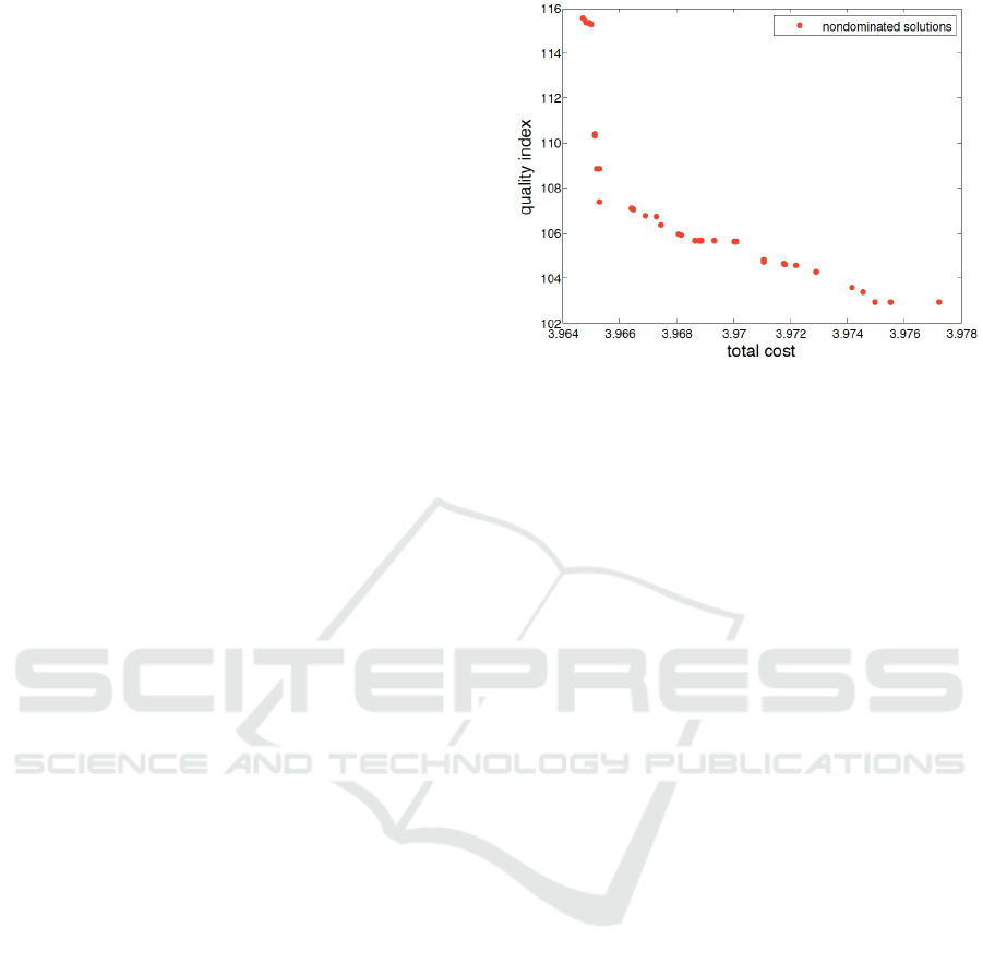
Figure 1: Trade-off curve for the total cost and quality in-

dex.

4.3 Results

This approach resulted in optimization problem with

2 objective functions, 115 decision variables being

bounded below and above, an inequality constraint

and 99 equality constraints. Due to a highly con-

strained search space, ﬁrst a feasible solution was

found. For this, 30 independent runs of EMyO/C were

performed setting µ = 1000, g

max

= 1000, CR = 0.15,

= 20 and p

= 1/n. Then, the best found solu-

tion among all the runs was improved by a single-

objective optimizer, HGPSAL (Esp

ırito Santo et al.,

2010). In order to obtain a set of Pareto optimal solu-

tions, another 30 independent runs of EMyO/C were

performed setting µ = 300, g

max

= 300 and introduc-

ing the obtained feasible solution into the initial pop-

ulation.

Figure 1 depicts all nondominated solutions ob-

tained after the performed experiments. The values of

the TC are in millions of euros (M e). In this ﬁgure,

the compromise solutions representing trade-offs be-

tween the total cost (TC) and quality index (QI) are

plotted. It can be seen that the proposed approach to

the WWTP design produces results with a physical

meaning. Speciﬁcally, the lower values of the qual-

ity index can be achieved through the increase in the

total cost, while the smaller values of the total cost re-

sult in the larger amount of pollution in the efﬂuent,

measured by the quality index.

In Table 1, the objective values along with the

most important decision variables of the obtained

trade-off solutions are presented, namely, the aeration

tank volume (V

), the air ﬂow rate (G

), the sedimen-

tation area (A

), the settler tank depth (h), the total

nitrogen (N), the chemical oxygen demand (COD),

and the total suspended solid (T SS). The presented

solutions are obtained after applying clustering pro-

Wastewater Treatment Plant Design: Optimizing Multiple Objectives

331

Table 1: Optimal values for the most important variables obtained using multiobjective approach.

h N COD T SS TC(M e) QI

100 6597.8531 271.7075 1 1.8982 125 10.7124 3.9647 115.5605

100 6598.438 271.7075 1 1.8982 125 10.4436 3.9649 115.3593

100 6598.9164 271.7075 1 1.3069 125 11.7056 3.9651 110.4133

100 6599.3342 271.7075 1 1.0247 125 11.7056 3.9653 108.8466

100 6599.363 271.7075 1.0637 0.90931 125 10.8241 3.9664 107.1068

100 6599.363 271.7075 1.0906 0.77282 125 10.8241 3.9669 106.7584

100 6599.363 271.7075 1.1116 0.83292 125 10.9469 3.9673 106.7376

100 6599.363 271.7075 1.1208 0.77282 125 10.8241 3.9674 106.3607

100 6599.363 271.7075 1.1598 0.71443 125 10.8241 3.9681 105.9032

100 6599.363 271.7075 1.1876 0.64562 125 10.82 3.9686 105.6695

100 6599.363 271.7075 1.1961 0.64562 125 10.82 3.9688 105.6695

100 6599.363 271.7075 1.2245 0.64562 125 10.82 3.9693 105.6695

100 6599.363 271.7075 1.2649 0.64562 125 10.7742 3.97 105.6352

100 6599.363 271.7075 1.3209 0.53704 125 10.8241 3.971 104.7857

100 6599.363 271.7075 1.3631 0.55629 125 10.8241 3.9718 104.6122

100 6599.363 271.7075 1.3835 0.55629 125 10.8241 3.9722 104.5415

100 6599.363 271.7075 1.4222 0.50336 125 10.8241 3.9729 104.2785

100 6599.363 271.7075 1.4924 0.32773 125 10.8241 3.9742 103.5757

100 6599.363 271.7075 1.5123 0.32773 125 10.8241 3.9745 103.3636

100 6599.363 271.7075 1.5359 0.32773 125 10.8241 3.9749 102.9405

100 6599.363 271.7075 1.5661 0.32773 125 10.8241 3.9755 102.9405

100 6599.363 271.7075 1.6586 0.34713 125 10.9389 3.9772 102.9399

cedure to group the data in the objective space. This

way, each solution represents a distinct cluster, hence

a different part of the trade-off curve. This procedure

allows to reduce the number of points, thereby facili-

tating the visualization of the results. Thus, different

design perspectives can be easily observed from the

obtained solutions.

It can be seen that the aeration tank volume and

the sedimentation area maintain the same values in

all the presented solutions. Only the slight variation

in a few solutions is observed concerning the air ﬂow

rate, whereas the settler depth has the larger variation

in the values between all the variables composing the

cost function. This hints that the lower cost as well as

the desirable values of the quality index can be mostly

achieved through controlling the settler depth. Fur-

thermore, it can be seen that the chemical oxygen de-

mand is at the highest allowable level (125), whereas

the total nitrogen and the total suspended solid are far

below the law limits (15 and 35, respectively).

Moreover, there is not a signiﬁcant difference in

the total cost in the various solutions, giving some

freedom in the design. For example, the QI in the

ﬁrst part of the solutions decreases signiﬁcantly for a

small increase in the TC.

5 MANY-OBJECTIVE APPROACH

In this section, the WWTP design is addressed by

simultaneously optimizing the most inﬂuential vari-

ables in the cost and quality index functions.

5.1 Results

To avoid the use of cost functions that are time and

local dependent, the variables inﬂuencing the invest-

ment and operation costs of a WWTP in each unit

operation are used as separate objectives. The vari-

ables that mostly inﬂuence the costs associated with

the aeration tank are the volume (V

) and the air ﬂow

). In terms of investment, the ﬁrst variable in-

ﬂuences directly the cost of the construction of the

tank, and the second inﬂuences the required power of

the air pumps. In terms of operation, both variables

will determine the power needed to aerate the sludge

properly, as well as the maintenance, in terms of elec-

tromechanical and civil construction material due to

deterioration. Assuming that the settling process is

only due to the gravity, the variables that most inﬂu-

ence the costs associated with the secondary settler

are the sedimentation area (A

) and the tank depth (h),

for obvious reasons.

Concerning the quality index function, each vari-

able on the right-hand side of (20) is considered as

a distinct function, thereby adding to the optimiza-

tion problem six different objectives. In contrast to

the previous formulation, this approach resulted in

the optimization problem with 10 objective functions.

EMyO/C was applied to the resulting problem setting

µ = 300, g

max

= 750 while keeping the remaining pa-

rameters as in the previous experiments and introduc-

ing the feasible solution into the initial population.

ICORES 2018 - 7th International Conference on Operations Research and Enterprise Systems

332

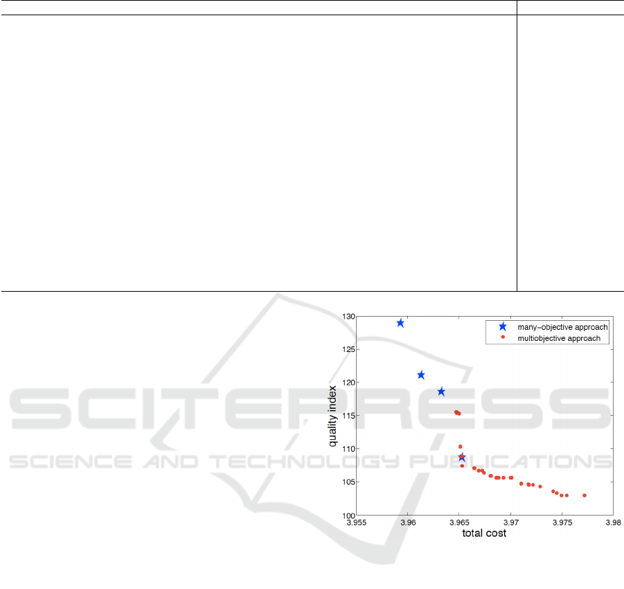
Table 2: Optimal values for the most important variables obtained using many-objective approach.

h N COD T SS BOD T KN S

e f

TC(M e) QI

100 6594.3023 271.7075 1 2.8161 124.2268 11.8656 61.1615 2.8064 0.0802 374.6088 3.9633 122.8764

100 6594.3023 271.7075 1 2.8171 124.1447 19.2583 61.0899 2.8064 0.0802 374.6306 3.9633 128.3383

100 6594.3023 271.7075 1 2.8453 124.3486 29.1979 57.9506 2.8064 0.0802 373.5855 3.9633 133.1374

100 6594.3023 271.7075 1 2.9506 124.2268 11.3468 61.2184 2.8064 0.0802 373.7916 3.9633 122.2631

100 6599.363 271.7075 1 3.2074 123.4647 34.0113 60.1686 3.2387 0.0802 373.2369 3.9653 141.1593

100 6589.2416 271.7075 1.3647 2.1974 125 19.7987 60.7109 1.9417 0.0802 373.4868 3.9678 121.9279

100 6594.3023 271.7075 1.3849 3.2028 123.374 25.6511 61.0103 3.2387 0.0802 374.5473 3.9702 135.9887

100 6599.363 271.7075 1.3036 2.4526 124.136 15.4315 60.4597 2.374 0.0802 373.1675 3.9707 121.2809

100 6599.363 271.7075 1.4351 3.2256 122.8556 34.5301 61.0103 3.2387 0.0802 374.0567 3.9731 142.2592

100 6594.3023 271.7075 1.5554 2.958 123.6176 15.4219 61.1504 2.8064 0.0802 373.6879 3.9733 124.9963

100 6599.363 271.7075 1.5061 2.106 124.5326 34.5059 60.7304 1.9417 0.0802 373.3003 3.9744 132.6874

100 6594.3023 271.7075 1.6622 2.1492 124.5326 12.1456 59.9099 2.374 0.0802 374.1559 3.9753 118.8802

100 6599.363 271.7075 1.5554 2.958 122.8556 30.1749 61.1504 2.8064 0.0802 374.2245 3.9753 135.9325

100 6599.363 271.7075 1.5558 2.4022 125 16.2075 60.6728 2.374 0.0802 373.0643 3.9753 122.3076

100 6594.3023 271.7075 1.6879 3.0518 123.6599 19.0348 60.8003 2.8064 0.0802 377.0701 3.9757 128.6042

100 6599.363 271.7075 1.6298 2.8089 122.904 32.9028 61.0551 2.8064 0.0802 373.848 3.9767 137.7822

100 6599.363 271.7075 1.6298 2.958 123.374 31.3109 60.5197 2.8064 0.0802 373.3762 3.9767 136.1953

100 6599.363 271.7075 1.6879 2.9973 123.9122 19.0348 60.8003 2.8064 0.0802 373.27 3.9777 127.4023

100 6589.2416 271.7075 1.9295 3.2703 124.6942 19.2583 61.6308 2.8064 0.0802 373.3365 3.9782 128.504

100 6594.3023 271.7075 1.927 2.8689 124.3001 13.7515 60.7982 3.2387 0.0802 373.5766 3.9802 126.933

The obtained set of nondominated solutions was

reduced by the clustering procedure applied in the ob-

jective space. Table 2 presents the most important

variables and the objective function values for a rep-

resentative of each cluster. Additionally, the values

of the total cost (TC) and the quality index (QI) were

calculated for these solutions. From the table, it can

be seen that the values of the aeration tank volume,

the sedimentation area as well as the nitrate and ni-

trite nitrogen are constant for all the presented solu-

tions. The values of the chemical oxygen demand are

slightly reduced compared with that obtained using

the multiobjective approach. On the other hand, the

values of the total nitrogen and the total suspended

solids are higher than in the previous experiments.

However, they are still below the law limits. Rela-

tively small variations can be observed regarding the

other variables, namely, the biochemical oxygen de-

mand, the total nitrogen of Kjeldahl and the efﬂuent

ﬂow.

Furthermore, the values of the total cost and the

quality index for all obtained nondominated solutions

were calculated. This way, a more general approach,

which only consists in minimizing the inﬂuential vari-

ables, is available to the particular case of the de-

sign of a WWTP facility. As a result, only four non-

dominated solutions were obtained in the space de-

ﬁned by TC and QI. These solutions along with all

nondominated solutions obtained using multiobjec-

tive approach are shown in Figure 2. It is interesting

to note that the range of the trade-off curve obtained

in the previous experiments was extended. The so-

lution with the smallest cost function value was ob-

Figure 2: Trade-off curves obtained using multiobjective

and many-objective approaches.

tained using the many-objective approach. This can

be explained by the fact that in a high dimensional ob-

jective space the number of nondominated solutions

is usually larger than in smaller dimensional spaces.

This effect results in the propagation of the dissimi-

larities between solutions in the decision space. Typ-

ically, this is an undesirable feature that adversely af-

fects the performance of evolutionary multiobjective

optimization algorithms. However, the advantageous

side effect is that different regions of the search space

can be explored, which happens to be the case in the

herein described experiments. Thus, the obtained re-

sults show that the many-objective approach can be

useful not only during a draft project when the exact

data about design of a particular WWTP is not avail-

able, but also for ﬁnding optimal values in the later

Wastewater Treatment Plant Design: Optimizing Multiple Objectives

333

stages of the decision-making process. Deﬁning and

simultaneously optimizing different combinations of

objectives can enrich the ﬁnal set of the obtained al-

ternatives, which are eventually presented to the deci-

sion maker.

6 CONCLUSIONS

This study addressed the optimization of a WWTP

whose model parameters were estimated using real

Portuguese data. Two different approaches that can

be extended to any WWTP unit operation modelling

were considered. In the ﬁrst approach, the WWTP de-

sign is addressed through a biobjective optimization

problem that consists of minimizing the total cost and

the quality index functions. The second approach is

more suitable for a draft project, when the exact loca-

tion and time where the WWTP is to be built is still

unknown. This approach involves the simultaneous

minimization of the inﬂuential variables, resulting in

a ten-objective optimization problem.

The results obtained in this study clearly show that

the WWTP design can be effectively approached by

simultaneously optimizing multiple objectives natu-

rally associated with the problem. The achieved opti-

mal solutions are meaningful in physical terms and

are economically attractive. Investment and opera-

tion costs are highly inﬂuenced by the optimized vari-

ables, stressing the importance of optimization. Both

approaches to WWTP design provide a set of non-

dominated solutions that can be used to gain valuable

insights about the problem and possible decision mak-

ing alternatives. This information can help to elabo-

rate a ﬁrst version of the project and reﬁne important

design choices when the speciﬁc location and moment

in time are deﬁned.

ACKNOWLEDGEMENTS

This work has been supported by the Portuguese

Foundation for Science and Technology (FCT) in the

scope of the project UID/CEC/00319/2013 (ALGO-

RITMI R&D Center).

REFERENCES

Alex, J., Benedetti, L., Copp, J., Gernaey, K. V., Jepps-

son, U., Nopens, I., Pons, M. N., Rosen, C., Steyer,

J. P., and Vanrolleghem, P. (2008). Benchmark sim-

ulation model no. 1 (BSM1). Technical report, IWA

Taskgroup on Benchmarking of Control Strategies for

WWTPs.

Deb, K., Pratap, A., Agarwal, S., and Meyarivan, T. (2002).

A fast and elitist multiobjective genetic algorithm:

NSGA-II. IEEE Trans. Evol. Comput., 6(2):182–197.

Denysiuk, R., Costa, L., and Esp

ırito Santo, I. (2013).

Many-objective optimization using differential evolu-

tion with variable-wise mutation restriction. In Proc.

Genet. Evol. Comput. Conf., pages 591–598.

Denysiuk, R., Costa, L., and Esp

ırito Santo, I. (2014).

Clustering-based selection for evolutionary many-

objective optimization. In Bartz-Beielstein, T.,

Branke, J., Filipi

c, B., and Smith, J., editors, PPSN

XIII, volume 8672 of LNCS, pages 538–547.

Denysiuk, R. and Gaspar-Cunha, A. (2017a). Multiob-

jective evolutionary algorithm based on vector angle

neighborhood. Swarm Evol. Comput., 37:45–57.

Denysiuk, R. and Gaspar-Cunha, A. (2017b). Weighted

stress function method for multiobjective evolutionary

algorithm based on decomposition. In Trautmann, H.,

Rudolph, G., Klamroth, K., Sch

utze, O., Wiecek, M.,

Jin, Y., and Grimme, C., editors, EMO, volume 10173

of LNCS, pages 176–190.

Esp

ırito Santo, I. A. C. P., Costa, L., Denysiuk, R., and Fer-

nandes, E. M. G. P. (2010). Hybrid genetic pattern

search augmented Lagrangian algorithm: Application

to WWTP optimization. In Proc. Conf. on Applied

Oper. Res., pages 45–56.

Esp

ırito Santo, I. A. C. P., Fernandes, E. M. G. P., Ara

ujo,

M. M., and Ferreira, E. C. (2006). On the secondary

settler models robustness by simulation. WSEAS

Transactions on Information Science and Applica-

tions, 3:2323–2330.

Henze, M., Jr, C. P. L. G., Gujer, W., Marais, G. V. R.,

and Matsuo, T. (1986). Activated sludge model no. 1.

Technical report, IAWPRC Task Group on Mathemat-

ical Modelling for design and operation of biological

wastewater treatment.

Miettinen, K. (1999). Nonlinear multiobjective optimiza-

tion, volume 12 of International Series in Operations

Research and Management Science. Kluwer Aca-

demic Publishers.

Tyteca, D. (1976). Cost functions for wastewater con-

veyance systems. J. Water Pollut. Control Fed.,

48(9):2120–2130.

Zeng, G.-M., Zhang, S.-F., Qin, X.-S., Huang, G.-H., and

Li, J.-B. (2003). Application of numerical simulation

on optimum design of two-dimensional sedimentation

tanks in the wastewater treatment plant. J. Environ.

Sci., 15(3):346–350.

Zhang, Q. and Li, H. (2007). MOEA/D: A multiobjective

evolutionary algorithm based on decomposition. IEEE

Trans. Evol. Comput., 11(6):712–731.

Zitzler, E. and K

unzli, S. (2004). Indicator-based selection

in multiobjective search. In Yao, E. K., Burke, J. A.,

Lozano, J., Smith, J. J., Merelo-Guerv

os, J. A., Bul-

linaria, J. E., Rowe, P., Ti

no, Kab

an, A., and Schwe-

fel, H.-P., editors, PPSN VIII, volume 3242 of LNCS,

pages 832–842.

ICORES 2018 - 7th International Conference on Operations Research and Enterprise Systems

334