
Heuristics for Improving Trip-Vehicle Fitness in On-demand
Ride-Sharing Systems
Sevket G¨okay
1,2
, Andreas Heuvels
1,2
and Karl-Heinz Krempels
1,2
1
Informatik 5 (Information Systems), RWTH Aachen University, Aachen, Germany
2
CSCW Mobility, Fraunhofer FIT, Aachen, Germany
Keywords:
Demand-Responsive Transport, Dial-a-Ride Problem with Time Windows, Ride-Sharing.
Abstract:
On-demand ride-sharing services are emerging alternatives to classical transport modes. Combined with self-
driving vehicles, this movement has potential to shape the future of our mobility. To make full use of the
potential, such services need to be scalable with growing demand. Assigning real-time trip requests to vehi-
cles such that the driving costs are minimized is computationally expensive, but has to be done fast. This
work proposes an approach to reduce the processing time it takes to assign a trip request to a vehicle. The
solution is a trip-vehicle fitness esti mation framework that is flexible enough to utilize any fitness measure and
is self -adjusting through feedback loops. We analyze the placement of a trip request within a vehicle schedule,
present and implement three fitness measures. The resulting system is evaluated based on performance, cus-
tomer satisfaction and vehicle costs criteria by running simulations. The evaluation results indicate si gnificant
performance improvement and noticeable improvements in terms of customer satisfaction and vehicle costs.
1 INTRODUCTION
Personal transportation, both private and public, is es-
sential for the well-being of a society. Private trans-
portation is flexible (w. r. t. time and location) and
convenient since it imposes n o vehicle ch a nges as in
its public counterpart. But it comes with traffic conge-
stion, parking place problems, increased gas emissi-
ons and additional costs attached to owning a vehicle.
Public transportation is usually cheaper and elimina-
tes the parking place problem, but is not as flexible
and c onvenient. Moreover, the quality of the service
can be poor in rural areas compared to urb a n areas. In
this Internet-driven informa tion age, classical systems
are being challenged by n ew ideas that take advantage
of in formation technology (IT) and the collective vi-
sion hints at a paradigm shift toward s Mobility-as-a-
Service (MaaS) where two trends meet: On-demand
shared mobility and self-driving vehicles (Greenblatt
and Shaheen, 2015; IFT, 2015 ).
On-demand transportatio n serv ices pick up the cu-
stomers at their desired time and bring them from
any location to any location, and therefore offer an
emerging middle ground between private and public
transportation. Uber
1
and Lyft
2
are IT-embracing,
1
https://www.uber.com
2
https://www.lyft.com
rising alternatives to the classical example for on-
demand transportation, that is the taxi service. These
are functionality-wise similar to a taxi service: Each
vehicle services one trip request after another, se-
quentially. Furthermore, they also offer ride-sharing
(UberPOOL an d Lyft Line) where multiple trip reque-
sts are comb ined into one vehicle ride by picking up
or droppin g off another customer while servicing a
trip request. This turns the cla ssical taxi service into
a m ore efficient offering (better use of resou rces with
increasing demand) and has po te ntial for a larger scale
deployment. There are also companies that c oncen-
trate on providing a ride-sharing service such as Via
3
,
allygator shuttle
4
and CleverShuttle
5
. Since the cus-
tomers can benefit from, e. g., reduc ed prices, but also
should be able to tolera te some newly-introduced do-
wnsides (i. e. potentially increased waiting and ride
times), a delicate trade-off has to be made between
customer satisfaction and service/veh icle c osts, which
are inherently in opposition to e ach other. Hereafter,
customer satisfaction refers to the number of satisfied
trip requests, waiting and ride times. Likewise, ser-
vice/vehicle costs refer to the number of vehicles in
service, distances driven by vehicles and vehicle ca-
3
https://ridewithvia.com
4
https://www.allygatorshuttle.com
5
http://clevershuttle.org
Gökay, S., Heuvels, A. and Krempels, K.
Heuristics for Improving Trip-Vehicle Fitness in On-demand Ride-Sharing Systems.
DOI: 10.5220/0006690203230334
In Proceedings of the 4th International Conference on Vehicle Technology and Intelligent Transport Systems (VEHITS 2018), pages 323-334
ISBN: 978-989-758-293-6
Copyright
c
2019 by SCITEPRESS – Science and Technology Publications, Lda. All rights reserved
323

pacity utilization.
There are two variants of on-demand transporta-
tion services with respec t to how trip requests become
apparent to the system. While in offline solutions all
requests are known before service and vehicle sche-
dules do not c hange after calculation (later during ser-
vice), online solutions process requests as they app e ar
in real- time without knowledge about the future and
constantly upda te the route of vehicles during service.
The performance of an online on-deman d ride-
sharing system (i. e. how fast it processes the request
and finds a fitting vehicle or not) is particularly impor-
tant, since the customers are r equesting rides in real-
time and waiting for resp onses. While most of the
theoretical related work concentrates on the offline
variant, the online variant offerings of aforementioned
private companies are niche such that the performanc e
and scalability are not big concerns. This work identi-
fies shortcomings of an existing system (G¨okay et al.,
2017) and improves it in this regard. While Section 2
provides an overview of the research field, Section 3
motivates this work. It describes in detail how the
problem has been diagnosed by perfor ming a simu-
lation using a real data set, collecting and analyzin g
statistics. Section 4 explains the taken o ptimization
approa c h on an abstract level. The proposed solu tion
is a flexible framework that combines multiple me-
asures which can influence trip-vehicle assignments.
We identify three measures and integrate them into
the fr a mework. Section 5 presents the details of the
technical realization, as well as th e implementation
improvements that have been carried out to take the
optimization efforts further. Section 6 illustrates the
evaluation metho dology and results. We let the pre-
vious and the current, improved implementation per-
form a simulation using identical configuration and
data sets. We compare and discuss the outcome of
both versions. Finally, Section 7 concludes the paper.
2 RELATED WORK
On-demand ride-sharing addresses the dial-a-ride
problem (DARP) (Cordeau and Laporte, 2007) which
is a generalization of a number of problems such as
Pickup and Delivery Problem (PDP) (Savelsbergh and
Sol, 1995), Vehicle Routing Problem (VRP) (Laporte,
1992b) an d Traveling Salesman Problem (TSP) (La-
porte, 1992a). While TSP c onsiders only one ser-
ver (i. e. vehicle), VRP works with a fleet of vehi-
cles. VRP only considers deliveries to locations, whe-
reas in PDP, vehicles transport goods from pickup to
delivery locations. All three problems have variants
that consider time constraints by employing time win-
dows, i. e. location visits have to occur within given
time windows, (Savelsbergh, 1985; Cordeau et al.,
2001a ; Parragh et al., 2008). Most DARP models
already impose time windows, so we consider it as
part of the prob le m definition. The main difference of
DARP from TSP, VRP and PDP is the human per-
spective: These problems aim to minimize vehicle
route costs and maximize the number of satisfied re-
quests. DARP additionally aims to minimize custo-
mer waiting and ride time in order to ma ximize cus-
tomer satisfaction.
DARP has two configurations: Online or offline,
single- or multi-vehicle. In (Cor deau and Laporte,
2007), the autho rs show that earliest works conce n-
trate on offline single-vehicle DARP, most of the
work addresses offline multi-vehicle DARP and only
very few of the algorithms solve online multi-vehicle
DARP. We believe that online multi-veh ic le variant is
the most promising when considering real- time, real-
world practica l usage.
Since DARP generalizes TSP, determining an op-
timal solution is NP- hard (Coja-Ogh lan et al., 2 005;
Gørtz, 2006). Even though there are ex a ct algorithms
that can fin d op timal solutions, these either so lve sim-
plified DARPs by leaving some constraints out or
work on small to medium problem instanc es (Psaraf-
tis, 1983; Desrosiers et al., 198 6; Ropke et al., 2007).
Many exact algorithms use a branch-and-cut techni-
que (Lysgaard et al., 2004; Cordeau, 2006). However,
due to the need in practical applications, most rela -
ted work focuses o n development of heuristics and
metaheuristics. There are some techniques that are
widely used such as neighborhood search (Pisinger
and Ropke, 2007), tabu search (Cordeau et al., 2001b;
Attanasio et al., 2 004), simu la te d annealing (Baugh
et al., 1998), insertion heuristics (Jaw et al., 1986;
Madsen et al., 1995; Tsubouchi et al., 2010 ), and ge-
netic algorithms (Jorgensen et a l., 2007).
Solving DARP with big problem instanc es in a
performant and scalable way only recently started to
get attention. The work in (Alonso-Mora et al., 2017)
presents a solution app roach to online multi-vehicle
DARP that starts with a greedy solution and improves
it in c rementally. The authors evaluate the algo rithm
by using 1000, 200 0, 3000 vehicles and ∼3 million
trip requests (∼500,000 per day). The requests are
collected for a time period (i. e. 10–50 seconds) and
then assigned to vehicles in batch e s, which detracts
from its real-time ap plicability. Anoth e r algorithm,
presented in (Ota et al., 2017), is evaluated by proces-
sing ∼260 million trip requests using between ∼500
and ∼6500 vehicles. It provides good performance,
but r equires extraordinary resource s (i. e. a 1200 CPU
core cluster). Both works evaluate their appro aches
VEHITS 2018 - 4th International Conference on Vehicle Technology and Intelligent Transport Systems
324
with trips extracted from New York City taxi trip data
(2010–201 3)
6
.
3 MOTIVATION
Having developed the initial version of an online
multi-vehicle DARP solution approa ch in (G¨okay
et al., 2017) but tested it with only small problem in-
stances (10-70 vehicle s and up to 5000 trip requests),
we wanted to challenge the sy stem and run a simula-
tion test with the same data set (one day with 524, 845
trip requests) and similar configuration (3000 vehicles
each with a c a pacity of 10 and a time window of 5
min for pick-up and drop-off events) as presented in
(Alonso-Mora et al., 2017) . The simulatio n was not
finished even after two and half days (we stopped it
after processing 292,200 re quests).
The fact, that a requ e st data set of one day could
not be processed at the very worst within a day, im-
plies that the system cannot scale and is not applicable
for real-time, practical usage. This led us to investi-
gate the possible sources of the problem.
Problem Description
Our approach employs insertion heuristics: A request
consists of a pick-up and drop-off event. Eac h event
comprises of a location, a time window an d an ac-
tual time within the time window, that represents the
point of time when the location will be visited by the
vehicle
7
. The processing pipeline of a request con-
tains a first stage, that sorts the vehicles according to
vehicle-request fitness, and a second stage that itera-
tes the sorted list of vehicles, inserts the request into
the schedule of the considered vehicle and tries to ad-
just the schedule in a way that the detour caused by
this new req uest does not violate the time constraints
of existing requests. After satisfying time constraints,
it is checked whether this new schedu le violates the
capacity constraints of the vehicle. The request is as-
signed to the first vehicle that has n o violations. A
detailed description of the working principle, an d the
scheduling algorithm, can be found in (G¨okay et al.,
2017), which bases on (Tsubouchi et al., 2010) .
During the adjustment of the schedule, the order
of events is changed several times until finding a fe-
asible order without time constraint violations. Mo-
reover, changing the order of events (and thus loca-
tions) causes m a ny routing calculations to determine
6
https://databank.illinois.edu/datasets/IDB-9610843
7
Maximum ride time constraints are implied, since both
pick-up and drop-off events have time windows.
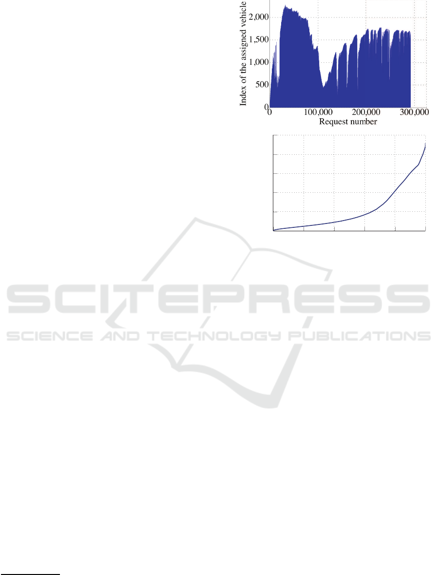
0
72.51
83.27 90.31
95.65
100
0
500
1,000
1,500
2,000
2,500
Percentile distribution (%)
Vehicle indices
Figure 1: Vehicle index statistics of the initial implemen-
tation for 292,200 requests with 3000 vehicles, vehicle
capacity of 10 and time window of 5 min (mean≈164,
stdev≈335, max=2281). The vehicle sorter is inefficient
about finding the fitting bus to which a request can be as-
signed.
the rid e times between newly ordered events so that
the algorith m can check whether time constrains are
still held . This many live routing calculations cau-
sed significant runtime overhead, since we do not pre-
compute and store the routes between all locations in
a lo okup table for the following reasons:
1. The boundaries o f the service area are defined
by the imported map during application startup,
which can be a s big as the service operato r desi-
res. Within the ser vice area the trip requests can
be made from any location to any loca tion. A pre-
defined set of allowed pick-up and drop-off loca-
tions would make pre-computatio n possible, but
also force customers to walk whic h is inconve-
nient.
2. Since the system is an online on-de mand service,
there is no knowledge a bout the future reque-
sts. Pre-computing routes from each location to
each location and storing them is only manageable
(w. r. t. computation space and time ) for offline va-
riants with small problem instan ces. At best, the
online system can cache computed routes to pre-
vent costly re-calcula tion of the same route. Our
implementation alrea dy utilizes route caches.
Heuristics for Improving Trip-Vehicle Fitness in On-demand Ride-Sharing Systems
325

Interestingly enough, most existing DARP solutions
neglect the route calculation cost aspect of the pro-
blem, since they consider the routes to be given, and
focus on the multi-criteria combinatorial optimiza-
tion. The aforementioned recent works, (A lonso-
Mora et al., 2017; Ota et al., 2017), utilize the gridlike
street geo graphy of Manhattan to pre-compute routes,
which is not the case for most service areas.
Having established that, we investigated whether
we can reduce the number of ro uting calculations.
The investigation led to the discovery that the first
stage in the pipe line, the vehicle sorter, was ineffi-
cient (Figure 1): The indices of the vehicles, to which
the requests were assigned, were so high within the
sorted vehic le list, that the second stage considered
many, ap parently unfitting, vehicles and thus has done
many unnecessary routing calculations.
4 APPROACH
Our optimization approach starts with the analysis
where pick-up and drop-off events are inserted into a
schedule. Figure 2 illustrates one section of a vehicle
schedule, in wh ich e
k−1
, e
k
, e
k+1
, e
k+2
are consecutive
events and the actual times are ord ered:
t
f irst
< ... < t
k−1
< t
k
< t
k+1
< t
k+2
< ... < t
last
When a new event e
new
has to be inserted into a sche-
dule, it should fall between two events, based on the
actual times of events: t
k
< t
new
< t
k+1
. We call the
position (i. e. the pair (e
k
, e
k+1
)), where the new event
e
new
falls, a pocket. While the schedule contained the
path e
k
→ e
k+1
before the insertion, afterwards it will
be changed to e
k
→ e
new
→ e
k+1
due to the detour.
The schedule of a vehicle contains the future re-
quests that are assigned to it. So, e
f irst
is the first
event that the vehicle has to service. Likewise, e
last
is
the last event in the schedule. An event cannot fall be-
fore the first event e
f irst
, because in this case it implies
that the event is in the past. In our implementation, a
vehicle is waiting idle at e
last
until a new request is
assigned to it (in the related pro blem spac e of VRP
the var iant, where vehicles are not required to return
to a depot afte r the last delivery, is called open VRP
(Li et al., 2007 )).
There are th ree possibilities where the pick-up and
drop-off events of a request might fall:
(P1) Both within the schedule (Figure 3a) :
t
f irst
< t
new
pick−up
< t
new
drop−o f f
< t
last
(P2) Pick -up in the schedule, drop-off after the
schedule (Figure 3b):
t
f irst
< t
new
pick−up
< t
last
< t
new
drop−o f f
e
k-1
e
k
e
k+1
e
k+2
e
new
(t
k-1
) (t
k
) (t
k+1
) (t
k+2
)
(t
new
)
e
first
(t
first
)
e
last
(t
last
)
Figure 2: Illustration of a pocket. T he event pair (e
k
, e
k+1
)
is the pocket for e
new
.
Since the dro p-off event does not fall into an
actual pocket, we treat (e
last
, e
new
drop−o f f
) as
such.
(P3) Both after the schedule (Figure 3c):
t
last
< t
new
pick−up
< t
new
drop−o f f
Since the pick-up event does not fall into an ac-
tual pocket, we treat (e
last
, e
new
pick−up
) as such.
To reduce the number of false positives of the vehicle
sorting stage an d therefore to have a more precise stra-
tegy, we incor porate the information w here the events
fall into our approach. Based on this observation, we
define three measures for sorting vehicles with respect
to a request for each event:
Detour Distance: This me asure ensures that we fa-
vor vehicles with minimal addition a l route costs
imposed by detours. It is calculated as the diffe-
rence between new and o ld path distance:
dist
e
k
→e
new
+ dist
e
new
→e
k+1
− dist
e
k
→e
k+1
However, the cases (P2) and (P3) contain situa-
tions in which the old path does not exist. We
address this issue in Section 4.1. Values returned
by this measure ar e treated as the lower the better.
Since we want the vehicle sorting stage to be fast,
we calculate all distances between two geolocati-
ons based on the haversine formula.
Largest Pocket: This measure e nsures that we disfa-
vor vehicles with p otential event constraint viola -
tions. Event constraint violations occur when the
actual times of two events are too close to each
other, while the locations of the events are too far
from each othe r. In such cases, our routing en -
gine calculates the shortest path duration from the
first to the subsequen t location and our scheduling
algorithm decid es that the vehicle cannot make it
to the subsequent event in time. Preventing these
cases redu ces the number of routing calcu lations.
Largest pocket is calculated as the division of time
available in pocket by the new path distan ce:
t
k+1
− t
k
dist
e
k
→e
new
+ dist
e
new
→e
k+1
VEHITS 2018 - 4th International Conference on Vehicle Technology and Intelligent Transport Systems
326
a
e
first
e
last
old
new
old
new
e
new
pick-up
e
new
drop-off
b
e
first
e
last
old
new
e
new
pick-up
e
new
drop-off
old
(missing)
new
c
e
first
e
last
old
(missing)
new
e
new
pick-up
e
new
drop-off
Figure 3: Possible event pockets: (a) Pick-up and drop-off events within the schedule (b) Pick-up in schedule, drop-off after
the schedule (c) Both events after the schedule
Values returned by this me asure are treated as the
higher the better.
Reward: Our vehicle sorting stage is intended to be
fast and therefore its calculations are approximate.
In the second stage, shortest path durations are
calculated and actual times are adjusted. This me-
asure ensures that we disfavor vehicles, where po-
tentially m ore event adjustments are needed, by
rewarding cases with less events within the sche-
dule. It assigns a constant value to ea c h case fol-
lowing the pr eference (P3) > (P2) > (P1) and va-
lues returned by this measure are treated as the
higher the better.
4.1 Old Path Distance Estimation
We define a mechanism to estimate old pa th distan-
ces in cases where we have only a new path distance
(drop-off in (P2) and pick-up in (P3)). For this, we
make use of the situatio ns, i. e. bo th events in (P1)
and pick-up event in (P2), where both the old and
new distances are present. Th e idea is to store and
always update th e average of old and new distance ra-
tios. Then, when it comes to e stima te the old p a th
distance, we multiply this ratio with the new path dis-
tance to a pproximate what the old path distance would
have been.
The distance values can be as small as tens of me-
ters and can grow up to tens of kilometers. Therefor e,
having only one ratio for the whole value spec trum
would not have b een precise. In order to handle the ra-
tios better, we divide the spectrum into multiple buc-
kets that are 200m wide.
4.2 Combining Measures
After establishing the basic building blocks of our ap-
proach , this section presents how we put everything
together. The optimiz ed vehicle sorter follows these
steps for each trip request and for each vehicle:
1. Determine the pockets for pick-up and drop-off
events, i. e. find out the case ((P1), (P2) or (P3))
for this request-schedu le mapping .
2. Calculate the three measures for this request-
schedule mapping.
3. Constru c t the weigh te d linear combination of the
three measures to derive the final fitness score.
4. Sort vehicles by their fitness sco re.
In the field of forecasting, the weights for combining
the features are commonly determined by incorpor a -
ting domain knowledge of experts and analyzing his-
torical data (Adya et al., 2001). One problem with
weighting is that past data may not reflect the current
characteristics a nd therefore using static weights can
result in poor accu racy (Miller et al., 1992) . We get
around this problem by employing a feedback mecha-
nism into our processing pipeline in order to inform
the vehicle sorter after processing each request how
good or bad the sorting was based on the index of the
assigned vehicle (Figur e 4). This approach can be de-
fined as dynamic linear combination (Lobrano et al.,
2010). In addition to sorting vehicles after the linear
combination step, we also sort vehicles by each mea-
sure, separately. By this means, we can compare the
global index a vehicle receives with the index ea ch
measure gave the same vehicle . If the measure gave
the vehicle a smaller (or higher) index than the final
index, the measure increases (or decreases) its weight.
Moreover, adjusting the weights based on only the
Heuristics for Improving Trip-Vehicle Fitness in On-demand Ride-Sharing Systems
327
Scheduler / Router
Try next
vehicle
Violates
constraints
No violation
Request
Processor
Vehicle Sorter
User
Notification
Vehicle / Driver
Notification
Reached
max retries
Feedback: Success
Feedback: Failure
Figure 4: Overview of the general framework how the trip
requests are processed with the added feedback mechanism.
last reque st or all past requests would be misleading,
since we rather want to recognize a trend and adjust
accordin gly. I n order to realize this, we use a moving
average of last 1000 indices for each measure.
4.3 Request Rejection Costs
Another important aspect is the processing costs of a
request rejection. A rejection means iterating all the
vehicles in the fleet, where no vehicle is a valid can-
didate for accepting the request into schedule. Wh en
the number of vehicles is huge, it takes an excessive
amount of time to reject a single request. With the
optimization tec hniques illustrated thus far, the im-
proved vehicle sorting stage p roduces less deviation
between the indices of assigned vehicles. We use this
outcome to our advantage and employ a filter to re-
duce the number vehicles that are to be considered.
We keep track of vehicle indices fo r accepted re que-
sts and update the moving average for subsequent re-
quests. The average index is used as a cut-off point
when the second stage iterates th e sorted list of vehi-
cles. T he average index is relaxed with each rejected
request, since it could mean that the cut-off point was
set too greedily.
5 IMPLEMENTATION
The system is developed as a standalone Java 8 ap-
plication. It uses GraphHopper
8
as the routing en-
gine, since it can be embedded into a Java application.
GraphHopper imports OpenStreetMap (OSM)
9
maps
and builds the underlying g raph to be used for routing.
Moreover, GraphHopper utilizes contraction hierar-
chies to speed up routing and we specify the transp or-
tation m ode as car. The com puted routes are easily
cacheable, because the g raph is not time-dependent
(as it would be in the case of public transportation
modes such as bus or train).
We make use of parallelization at all steps where
it is possible. One step worth mentioning is the se-
cond stage, the scheduler in Figure 4. The initial im-
plementation iterated the list of vehicles sequentially.
This takes too lon g, if the viable vehicle has a high
index in the list. Parallel processing with paralleliza-
tion factor set to th e number of vehicles to be con sid e-
red can also be c ostly due to context switching, if this
number is h uge. We pa rtition the sorted list of vehi-
cles in to batches with size set to the number of CPU
cores of the system. The scheduler runs for each vehi-
cle within a batch in parallel. If no viable vehicle is
found in this batch, we continue with the next batch.
If there are resu lts, we calculate th e total time cost for
each result and pick the vehicle with the lowest cost,
which is determined by the sum of several criteria:
• I ncreased costs of the vehicle
∆
v
= travelTime(S
new
) − travelTime(S
prev
),
where travelTime(S) is the sum of all trips in
schedule S.
• I ncreased costs for ea c h customer due to the sche-
dule adjustment
∆
S
=
∑
c ∈ S
new
cost
S
new
(c) −
∑
c ∈ S
prev
cost
S
prev
(c),
where cost
S
(C) denotes the cost for a customer C
in schedule S and is calculated as the sum of wai-
ting and ride time.
6 EVALUATION
We perform two simu la tions, one with the old and
one with the new vehicle sorting strategy implemen-
tation, u sin g the same simulation configuration and
data sets, and compare their results. The old vehi-
cle sorting strategy is the one presented in (Tsubouchi
8
https://www.graphhopper.com/
9
http://www.openstreetmap.org/
VEHITS 2018 - 4th International Conference on Vehicle Technology and Intelligent Transport Systems
328
et al., 2010), which prefers vehicles with the c losest
direction to the new trip request. Both simulations
benefit from the improvements outlined in Section 5.
The simulations are run inside a virtual machine con-
figured with 8 vCPUs (Intel Xeon E5-2650 clocked at
2.20 GHz) a nd 8 GB system memory. Used Java Vir-
tual Machine parameters are
-Xms2048m -Xmx4096m
-XX:+UseG1GC
. As of writing, this system configura-
tion represents an entry level off-the-shelf server.
The OSM data used for New York City con-
tains all infor mation and changes up to 2017-04-
09T15:01:34Z . We extra c t tr ips from New York City
taxi trip data (2010– 2013) for the day Satur day May
11, 2013 (524,845 trips after clea n-up). From each
data point we read the pick-up date time (we treat this
as the beginning of the pick-up time window) and the
geolocatio ns o f pick-up and drop-off to construc t the
trip requests. Number of passengers is set to 1. Since
the previous vehicle sorting strategy could not cope
with processing all trips of a d ay in reasonable time,
we prepare three data sets:
1. Reduced number of trips by selecting every 10th
(from 00:00 to 2 3:59 totaling to 52,552 trips). The
aim is to keep the distribution as close as possible
to Figure 5 with less data points. Hereby, we as-
sume not to introduce a selection bias.
2. Picking a tim e interval with high density of reque-
sts to represent peak demand (with pick-up times
from 19:00 to 20:00 totaling to 30,88 4 trips)
3. Picking a time interval with low density of reque-
sts to represent off-peak demand (with pick-up ti-
mes from 05:00 to 07:00 totaling to 10,388 trips).
The configuration consists of number of vehicles (d e-
pending on the data set this parameter varies between
100 and 3000), vehicle capacity (3 or 10) and time
window (5 or 10 min). For all data sets, all vehicles
are initialized at the same location and at the start of
the data set’s time range ( e . g. for low d ensity data
set at 05:00). We evalu ate our results in three cate-
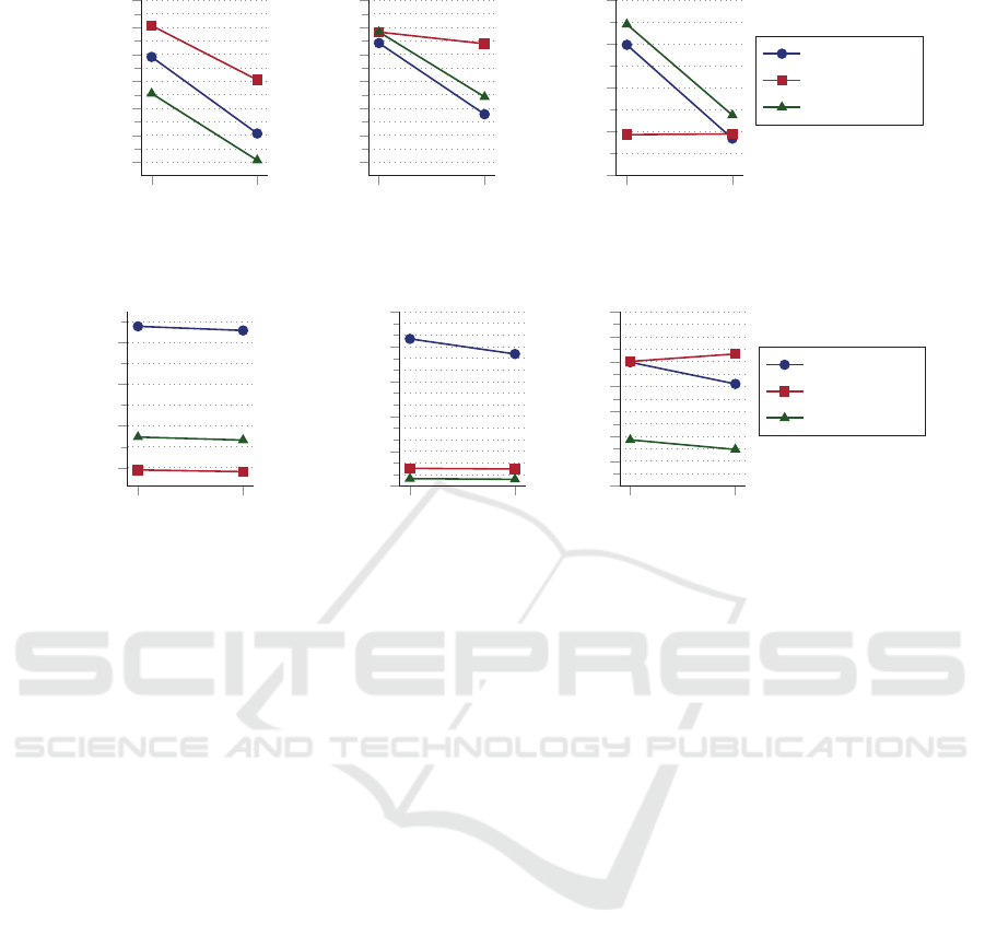
gories: Performance improvement (Figure 6), custo-
mer satisfaction (Figure 7) an d service/vehicle costs
(Figure 8). We also discuss how the changes aiming
at performan c e improvemen ts affect the customer sa-
tisfaction and service costs. The de ta iled results are
presented in Tables 1 and 2.
Figure 6 shows that the improved implementation
is always faster in terms of request-vehicle assign -
ment calculation duration. The average calculation
duration is reduced from 27 07 ms to 320 ms (worst
case). This is due to the fact that it co nsiders less false
positive vehicles until finding a v ia ble vehicle for a
request (i. e. redu c ed average vehicle index). This im-
proves the total run time substantially (Table 1). As
01:00
04:00
08:00
12:00
16:00
20:00
23:00
5
10
15
20
25
30
35
·10
3
Time of day
Trip count
Figure 5: Hourly trip distribution throughout the day on Sa-
turday May 11, 2013.
new
old
0
50
100
150
200
250
300
350
400
Avg vehicle index
every 10th
low density
high density
new
old
0
250
500
750
1,000
1,250
1,500
1,750
2,000
2,250
2,500
2,750
Avg calculation duration (in ms)
Figure 6: Performance comparison of the old and new i m-
plementation. Average vehicle index is reduced, since the
new implementation considers less false positives. This
significantly reduces the calculation duration of request-
vehicle assignments.
can be seen in Figure 7, the customer satisfactio n as-
pect benefits fr om improved implementation. We can
recogn ize that the new version alm ost always reduces
the waiting time and r ide delay of cu stomers while
producing similar or better success rate
10
. Ride de-
lay improvements are n ot that prominent or slightly
worse with the low density data set, because the new
implementation consistently has higher success rate
(see Table 2).
These improvements can come at slightly increa-
sed vehicle costs. Vehicle statistics in Tab le 2 show
that the new implementation has somewhat higher
vehicle costs when th e c onfiguration is too generous
(e. g. more vehicles in service than actually needed),
because it distributes requests more evenly across a ll
10
The number of accepted requests divided by the num-
ber of all requests
Heuristics for Improving Trip-Vehicle Fitness in On-demand Ride-Sharing Systems
329
new
old
1
1.4
1.8
2.2
2.6
3
3.4
Avg wait time (in min)
new
old
1
1.4
1.8
2.2
2.6
3
3.4
Avg ride delay (in min)
new
old
1.3
1.4
1.5
1.6
1.7
Avg ratio of actual
to direct ride time
every 10th
low density
high density
Figure 7: Customer satisfaction comparison of the old and new implementation. Both wait time and ride delay are lower with
the new implementation. Average ratio of actual to direct ride time expresses the relative ride delay.
new
old
5
10
15
20
·10
4
Total distance (in km)
new
old
0
250
500
750
1,000
1,250
Avg distance per
vehicle (in km)
new
old
15
20
25
30
35
40
45
50
Avg capacity util. (%)
every 10th
low density
high density
Figure 8: Service/vehicle costs comparison of the old and new implementation. Average capacity utilization decreases with the
data sets every 10th and high density because with some simulation configurations the new implementation is at a disadvantage
(see Table 2).
vehicles (as highlighted by the column # of used veh i-
cles). Even though the driven distan ce per vehicle is
lower, there ar e more vehicles that are used. This si-
tuation results in a slightly higher sum of driven dis-
tance of all vehicles. Moreover, we capture capacity
utilization statistics for each customer-vehicle assig-
nment by counting total customers in a vehicle after
picking up the new customer. Figure 8 illustrates tha t
average capacity utilization decreases with the data
sets every 10th an d high density. This is due to the
huge differences between the new and old implemen-
tation with generous configurations. Sin ce the events
in vehicle schedules are not tha t dense with the new
implementation (a conseq uence of even distribution
of requests to all vehicles), capacity utilization is lo-
wer. Even though the new implementation yields bet-
ter capa city utilization results with diminishing con-
figuration s, they are not d ominant enough to counter-
balance the overall average. With diminishing con-
figuration s the new implementation starts to produce
better results in all aspects. If the number of vehicles
is set to a value such that both implementations have
to make use of all the vehicles, then in most cases
the new implementation satisfies more customers (i. e.
achieves higher success rate) with less vehicle costs.
As a result, the total distance driven by all vehicles or
the average distance driven per vehicle stays more or
less the same (Figure 8).
7 CONCLUSION
On-demand r ide-sharing systems are becoming incre-
asingly p opular. This entails a potential scalibility
problem which only recently started to get attention.
In th is work, we presented an optimization approach
for an online on-d emand ride-sharing system that was
intended to be a runtime improvement without sacri-
ficing quality of the results, but the evaluation showed
that the new approach can yield better results as we ll.
The system’s working principle consists of a trip re-
quest processing pipeline with two stages. The first
stage, the vehicle sorter, sorts th e vehicles according
to their requ e st-veh ic le a ssignment fitness. The se-
cond stage, the scheduler, iterates the list of sorted
vehicles an d adjusts the schedule of each vehicle (af-
ter inserting the new request into the schedule) such
that the detours imposed by the inclusion of the new
request do not break the time constraints of othe r re-
quests. Sche dule adjustments include a large number
of routing calculations which are costly. The schedu-
ler iterates the list until finding one viable vehicle that
can tolerate the inclusion of the new request and to
which the request is assign ed. The need for a runtime
improvement is based on the evalua tion with huge
data sets (∼500,000 trip requests) and thousands of
vehicles. The evaluation took such a long time to
VEHITS 2018 - 4th International Conference on Vehicle Technology and Intelligent Transport Systems
330

process the requests, that the so lution was not appli-
cable for rea l-time usag e. We identified th at the cause
of this problem was the former vehicle sorting stage,
which inefficiently considered false p ositive vehicles
as fitting and therefore the second stage, the schedu-
ler, had to do many schedule adjustments of unfitting
vehicles.
The pro posed optimization replaces the vehicle
sorting stage and tries to avoid time constraint vio-
lations. At first, we determine the pockets (i. e. po-
tential placements) of the pick-up and drop-off events
of a new request within a schedule and use the infor-
mation gathered from n eighboring events for a mo re
precise ju dgment. Based on this, we calculate thre e
measures (detour distance, largest pocket and reward)
and derive the final fitness score by the weighted li-
near combination of these three measures. Moreover,
we introduc e a feedback loop into the processing pi-
peline for the system to learn from its successes and
failures in order to regulate the measure weights ac-
cordingly. For the evaluation, we extract trip reque-
sts from New York City taxi trip data and run two
simulations, i. e., we let the old and new implementa-
tions with otherwise identical configurations process
the same re quests. The evaluation results are categori-
zed in three groups: Performance improvement, cus-
tomer satisfaction and serv ic e costs. As the main goal
of this work, the new implementation outperforms the
old one in all simulation s. Moreover, the new imple-
mentation provides better customer satisfaction in al-
most all simulations. Since the new implementatio n
aims to minimize the possibility of tim e constraint
violations, it distributes requests more evenly to all
vehicles. With generou s configurations (e. g. there
are more vehicles in service than actually needed), it
has slightly higher vehicle costs. When reducin g the
number of vehicles, the new implementation starts to
yield better results in all aspec ts. We observe that a
time wind ow of 10 min and 2000 vehicles each with a
capacity of 10 can satisfy 98% of the demand at peak
periods. At off-peak time perio ds, the n umber of vehi-
cles can be reduced to 500 to accomplish the same.
This work serves as a basis for fu rther experimen-
tation and improvements. Having a fast evaluation
cycle enables extensive testing with big problem in-
stances to better assess the real-world applicability.
Event tho ugh the performance gain is particularly evi-
dent with the data set high density, the test runtime is
still suboptimal with some c onfigurations. Further-
more, the disadvantageou s consequences of generou s
configurations (making use of all vehicles, decre a sed
shared rides and capacity utilization) should be avoi-
ded. Addressing these issues is part of future work.
ACKNOWLEDGMENTS
This work was partially fun ded by the Ger man Fe-
deral Ministry of Transport and Digital Infrastructure
(BMVI) for the project “Dig italisierte Mobilit¨at – die
Offene Mobilit¨atsplattform” (19E16007B).
REFERENCES
Adya, M., Collopy, F., Armstrong, J., and Kennedy, M.
(2001). Automatic identification of time series featu-
res for rule-based forecasting. International Journal
of Forecasting, 17(2):143–157.
Alonso-Mora, J., Samaranayake, S., Wall ar, A. , Fraz-
zoli, E., and Rus, D. (2017). On-demand high-
capacity ride-sharing via dynamic trip-vehicle assign-
ment. Proceedings of the National Academy of Scien-
ces, 114(3):462–467.
Attanasio, A., Cordeau, J.-F., Ghiani, G., and Laporte, G.
(2004). Parallel tabu search heuristics for the dyna-
mic multi-vehicle dial-a-ride problem. Parallel Com-
puting, 30(3):377 – 387.
Baugh, J. W., Kakivaya, G. K. R., and Stone, J. R. (1998).
Intractability of the dial-a-ride problem and a multiob-
jective solution using simulated annealing. Engineer-
ing Optimization, 30(2):91–123.
Coja-Oghlan, A., Krumke, S. O., and Nierhoff, T. (2005).
A Hard Dial-a-Ride Problem that is Easy on Average.
Journal of Scheduling, 8(3):197–210.
Cordeau, J.-F. (2006). A branch-and-cut algorithm for the
dial-a-ride problem. Oper. Res., 54(3):573–586.
Cordeau, J.-F., Desaulniers, G., Desrosiers, J., Solomon,
M. M., and Soumis, F. (2001a). VRP with Time Win-
dows. In Toth, P. and Vigo, D., editors, The Vehi-
cle Routing Problem, pages 157–193. Society for In-
dustrial and Applied Mathematics, Philadelphia, PA,
USA.
Cordeau, J.-F. and Laporte, G. (2007). The dial-a-ride pro-
blem: models and algorithms. Annals of Operations
Research, 153(1):29–46.
Cordeau, J.-F., Laporte, G., and Mercier, A. (2001b). A
unified tabu search heuristic for vehicle routing pro-
blems with time windows. Journal of the Operational
Research Society, 52(8):928–936.
Desrosiers, J., Dumas, Y., and Soumis, F. (1986). A
dynamic programming solution of the large-scale
single-vehicle dial-a-ride problem with time windows.
American Journal of Mathematical and Management
Sciences, 6(3-4):301–325.
G¨okay, S., Heuvels, A., Rogner, R., and Krempels, K.-H.
(2017). Implementation and Evaluation of an On-
Demand Bus System. In Proceedings of the 3rd Inter-
national Conference on Vehicle Technology and Intel-
ligent Transport Systems (VEHITS 2017), Porto, Por-
tugal.
Gørtz, I. L. (2006). Hardness of preemptive finite capa-
city dial-a-ride. In in C omputer Science, L. N., edi-
tor, Proceedings of 9th I nternational Workshop on Ap-
Heuristics for Improving Trip-Vehicle Fitness in On-demand Ride-Sharing Systems
331

proximation Algorithms for Combinatorial Optimiza-
tion Problems ( APPROX 2006).
Greenblatt, J. B. and Shaheen, S. (2015). Automated
vehicles, on-demand mobility, and environmental im-
pacts. Current Sustainable/Renewable Energy Re-
ports, 2(3):74–81.
IFT (2015). Urban Mobility System Upgrade – How
shared self-driving cars could change city traffic.
Research report, International Transport Forum at
the Organisation for Economic Co-operation and
Development (OECD). Available at https://www.itf-
oecd.org/sites/default/files/docs/15cpb
self-
drivingcars.pdf.
Jaw, J.-J., Odoni, A. R., Psaraftis, H. N., and Wilson, N. H.
(1986). A heuristic algorithm for the multi-vehicle
advance request dial-a-ride problem wi th time win-
dows. Transportation Research Part B: Methodolo-
gical, 20(3):243 – 257.
Jorgensen, R. M., Larsen, J., and Bergvinsdottir, K. B.
(2007). Solving the dial-a-ride problem using gene-
tic algorithms. Journal of the Operational Research
Society, 58(10):1321–1331.
Laporte, G. (1992a). T he traveling salesman problem: An
overview of exact and approximate algorithms. Eu-
ropean Journal of Operational Research, 59(2):231 –
247.
Laporte, G. (1992b). The vehicle routing problem: An over-
view of exact and approximate algorithms. European
Journal of Operational Research, 59(3):345 – 358.
Li, F., Golden, B., and Wasil, E. (2007). The open vehi-
cle routing problem: Algorithms, l arge-scale test pro-
blems, and computational results. Comput. Oper. Res.,
34(10):2918–2930.
Lobrano, C., Tronci, R., Giacinto, G., and Roli, F. (2010).
Dynamic Linear Combination of Two-Class Classi-
fiers, pages 473–482. Springer Berlin Heidelberg,
Berlin, Heidelberg.
Lysgaard, J., Letchford, A. N., and Eglese, R. W. (2004).
A new branch-and-cut algorithm for the capacitated
vehicle routing problem. Mathematical Program-
ming, 100(2):423–445.
Madsen, O. B. G., Ravn, H. F., and Rygaard, J. M. (1995). A
heuristic algorithm for a dial-a-ride problem with time
windows, multiple capacities, and multiple objectives.
Annals of Operations Research, 60(1):193–208.
Miller, C. M., Clemen, R. T., and Winkler, R. L. (1992).
The effect of nonstationarity on combined forecasts.
International Journal of Forecasting, 7(4):515 – 529.
Ota, M., Vo, H., Silva, C., and Freire, J. (2017). STaRS:
Simulating Taxi Ride Sharing at Scale. IEEE Tran-
sactions on Big Data, 3(3):349–361.
Parragh, S. N., Doerner, K. F., and Hartl, R. F. (2008).
A survey on pickup and delivery problems - Part I:
Transportation between customers and depot. Journal
f¨ur Betri ebswirtschaft.
Pisinger, D. and Ropke, S. (2007). A general heuristic for
vehicle routing problems. Computers & Operations
Research, 34(8):2403 – 2435.
Psaraftis, H. (1983). An exact algorithm for the single vehi-
cle many-to-many dial-a-ri de problem with time win-
dows. Transportation Science, 17(3):351–357.
Ropke, S., Cordeau, J.-F., and Laporte, G. (2007). Models
and branch-and-cut algorithms for pickup and delivery
problems with time windows. Networks, 49(4):258–
272.
Savelsbergh, M. and Sol, M. (1995). The general
pickup and delivery problem. Transportation Science,
29(1):17–29.
Savelsbergh, M. W. P. (1985). Local search in routing pro-
blems with time windows. Annals of Operations Re-
search, 4(1):285–305.
Tsubouchi, K., Yamato, H., and Hiekata, K. (2010). Inno-
vative on-demand bus system in Japan. IET Intelligent
Transport Systems, 4(4):270–279.
VEHITS 2018 - 4th International Conference on Vehicle Technology and Intelligent Transport Systems
332
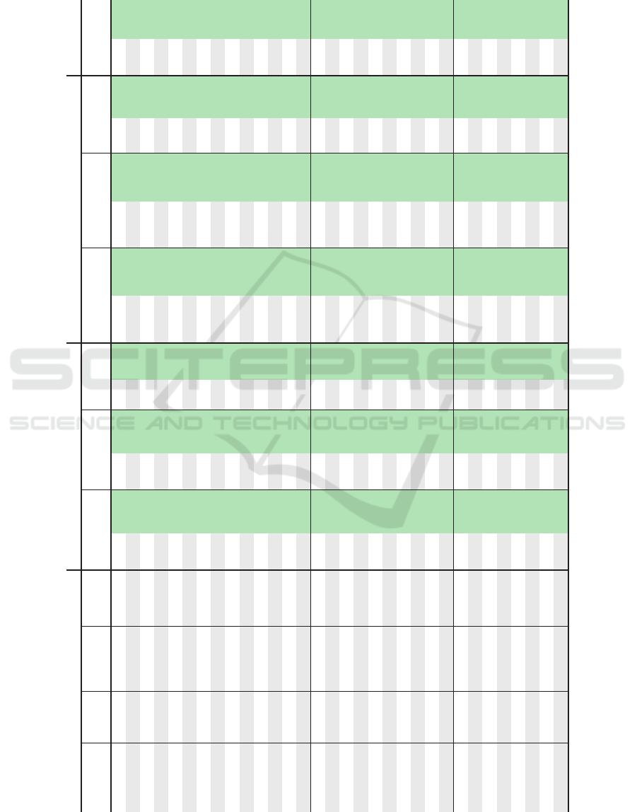
Table 1: Performance overview of test cases. Each cell contains a value that represents the result of the simulation with the
new implementation and another value within parentheses that expresses the difference of the this value from the result of the
simulation w ith the old implementation. The green (or red) cells indicate that the new implementation produced a better ( or
worse) result.
Test case setup Indices of assigned vehicles Calculation durations for each request (in ms)
Data set # of vehicles Vehicle capacity
Time window
(in min)
Mean Stdev Max Mean Stdev Max
Test runtime
(in h)
every 10th 500 10 10 1.22 ( −55.94) 0.81 ( −46.46) 8 ( −262) 4.86 ( −191.60) 2.24 ( −167.09) 91 ( −2718) 0.07 ( −2.80)
every 10th 500 10 5 1.27 ( −58.03) 0.86 ( −47.46) 8 ( −280) 4.96 ( −189.41) 2.41 ( −162.50) 78 ( −2559) 0.07 ( −2.76)
every 10th 500 3 10 1.21 ( −57.51) 0.80 ( −47.46) 8 ( −267) 4.82 ( −191.67) 2.11 ( −166.13) 73 ( −2730) 0.07 ( −2.80)
every 10th 500 3 5 1.30 ( −58.72) 0.89 ( −47.66) 8 ( −267) 5.02 ( −191.44) 2.46 ( −163.75) 98 ( −2481) 0.07 ( −2.79)
every 10th 250 10 10 2.84 ( −58.82) 2.61 ( −47.77) 32 ( −218) 17.44 ( −226.61) 16.54 ( −220.10) 245 ( −3084) 0.25 ( −3.31)
every 10th 250 10 5 4.17 ( −55.10) 4.04 ( −43.97) 50 ( −200) 23.54 ( −194.77) 21.91 ( −187.08) 326 ( −2351) 0.34 ( −2.84)
every 10th 250 3 10 3.59 ( −60.97) 3.44 ( −48.15) 42 ( −208) 19.70 ( −233.80) 18.70 ( −222.30) 349 ( −2626) 0.29 ( −3.41)
every 10th 250 3 5 4.06 ( −56.42) 4.13 ( −44.35) 54 ( −196) 22.57 ( −201.22) 22.69 ( −190.94) 318 ( −2841) 0.33 ( −2.94)
every 10th 175 10 5 5.73 ( −50.03) 6.05 ( −35.75) 79 ( −96) 52.94 ( −215.54) 66.30 ( −138.40) 664 ( −1857) 0.77 ( −3.15)
every 10th 175 3 5 5.97 ( −50.86) 6.41 ( −35.72) 95 ( −80) 55.93 ( −214.78) 68.63 ( −133.00) 704 ( −1705) 0.82 ( −3.14)
every 10th 100 10 10 7.97 ( −32.31) 8.66 ( −17.71) 59 ( −41) 94.95 ( −140.11) 66.29 ( −49.36) 825 ( −527) 1.39 ( −2.05)
every 10th 100 10 5 5.36 ( −32.17) 5.36 ( −20.45) 56 ( −44) 90.50 ( −131.09) 66.45 ( −47.32) 739 ( −676) 1.32 ( −1.91)
every 10th 100 3 10 8.15 ( −32.55) 8.81 ( −17.05) 63 ( −37) 94.11 ( −139.91) 64.53 ( −48.09) 620 ( −711) 1.37 ( −2.04)
every 10th 100 3 5 5.39 ( −32.81) 5.38 ( −20.55) 60 ( −40) 89.56 ( −132.29) 65.67 ( −47.10) 726 ( −791) 1.31 ( −1.93)
high density 3000 10 10 4.31 (−393.26) 3.05 (−382.55) 78 (−2385) 9.53 (−1850.68) 8.08 (−2048.44) 235 (−28 836) 0.08 (−15.88)
high density 3000 10 5 4.17 (−353.80) 3.16 (−352.93) 107 (−2078) 10.84 (−1639.17) 11.40 (−1898.11) 322 (−24 989) 0.09 (−14.06)
high density 2000 10 10 5.01 (−457.82) 2.76 (−434.98) 60 (−1940) 12.66 (−2977.16) 12.95 (−3485.42) 414 (−25 105) 0.11 (−25.54)
high density 2000 10 5 4.84 (−375.56) 3.41 (−379.04) 99 (−1901) 17.80 (−2049.96) 19.73 (−2692.67) 271 (−24 320) 0.15 (−17.58)
high density 1500 10 10 4.50 (−432.18) 2.71 (−381.56) 45 (−1455) 20.03 (−3474.81) 17.66 (−3327.30) 267 (−18 772) 0.17 (−29.81)
high density 1500 10 5 11.44 (−371.43) 22.10 (−338.67) 301 (−1199) 106.96 (−2819.85) 256.50 (−2788.13) 2775 (−16 664) 0.92 (−24.19)
high density 1250 10 10 18.62 (−372.60) 41.91 (−290.92) 477 ( −773) 546.16 (−2874.99) 1071.62 (−1833.93) 6587 ( −9732) 4.68 (−24.66)
high density 1250 10 5 19.12 (−330.01) 31.86 (−286.81) 465 ( −785) 516.76 (−2464.63) 853.35 (−1821.24) 5299 (−10 876) 4.43 (−21.14)
high density 1000 10 10 26.24 (−302.14) 49.13 (−223.95) 515 ( −485) 1064.31 (−1909.83) 1314.02 ( −897.47) 6655 ( −6080) 9.13 (−16.38)
high density 1000 10 5 18.86 (−279.96) 28.61 (−233.94) 376 ( −624) 888.25 (−1817.94) 1068.72 (−1017.07) 5043 ( −8092) 7.62 (−15.59)
low density 500 10 10 4.42 (−145.12) 2.93 (−121.60) 22 ( −478) 22.45 ( −747.65) 18.64 ( −596.09) 437 ( −3588) 0.06 ( −2.16)
low density 500 10 5 12.39 (−136.96) 17.88 (−105.74) 199 ( −301) 110.63 ( −618.04) 169.06 ( −380.36) 1481 ( −2342) 0.32 ( −1.78)
low density 500 3 10 8.88 (−148.04) 11.32 (−112.75) 155 ( −345) 50.27 ( −745.42) 84.76 ( −515.78) 856 ( −2825) 0.15 ( −2.15)
low density 500 3 5 13.57 (−139.01) 19.29 (−106.86) 214 ( −286) 122.25 ( −608.67) 176.22 ( −372.48) 1426 ( −2149) 0.35 ( −1.76)
low density 250 10 10 12.48 ( −74.18) 17.59 ( −49.66) 133 ( −117) 239.66 ( −346.40) 181.12 ( −103.61) 943 ( −757) 0.69 ( −1.00)
low density 250 10 5 11.23 ( −72.56) 14.97 ( −49.80) 149 ( −101) 230.23 ( −315.45) 165.81 ( −104.03) 748 ( −970) 0.66 ( −0.91)
low density 250 3 10 13.80 ( −75.61) 18.24 ( −48.01) 141 ( −109) 242.78 ( −343.95) 173.74 ( −103.24) 938 ( −724) 0.70 ( −0.99)
low density 250 3 5 10.68 ( −75.48) 14.24 ( −51.25) 141 ( −109) 232.70 ( −315.65) 169.40 ( −91.04) 959 ( −990) 0.67 ( −0.91)
Heuristics for Improving Trip-Vehicle Fitness in On-demand Ride-Sharing Systems
333
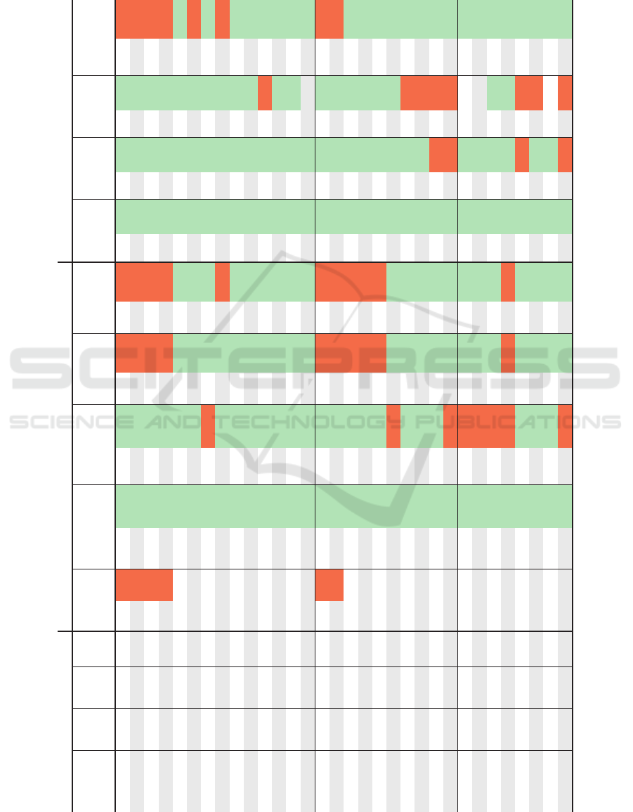
Table 2: Statistics w. r. t. vehicle/service costs and customer satisfaction. Each cell contains a value that represents the result of
the si mulation with the new implementation and another value within parentheses that expresses the difference of the this value
from the result of the simulation with the old implementation. The green (or red) cells indicate that the new implementation
produced a better (or worse) result.
Test case setup Vehicle/service costs Customer satisfaction
Data set
# of
vehicles
Vehicle
capacity
Time
window
(in min)
# of used
vehicles
Mean driven
distance per
vehicle (in km)
Stdev driven
distance per
vehicle (in km)
Shared rides
(%)
Avg capacity
util (%)
Avg waiting
time (in min)
Avg ride
delay (in min)
Avg ratio of
actual to direct
ride times
Success rate
(%)
every 10th 500 10 10 500 (+155) 607.88 (−211.80) 43.58 (−355.50) 2.57 (−59.73) 10.27 ( −9.54) 0.05 (−3.04) 0.12 (−3.72) 1.11 (−0.76) 99.85 ( −0.14)
every 10th 500 10 5 500 (+166) 607.87 (−200.56) 44.09 (−366.71) 2.49 (−54.98) 10.26 ( −8.02) 0.04 (−1.86) 0.09 (−2.09) 1.08 (−0.45) 99.76 ( −0.16)
every 10th 500 3 10 500 (+140) 608.51 (−196.46) 44.91 (−360.39) 2.46 (−60.74) 34.22 (−29.00) 0.05 (−3.04) 0.11 (−3.71) 1.11 (−0.76) 99.86 ( −0.13)
every 10th 500 3 5 500 (+159) 607.93 (−189.41) 43.49 (−373.54) 2.56 (−54.88) 34.23 (−25.16) 0.04 (−1.86) 0.09 (−2.06) 1.08 (−0.44) 99.75 ( −0.17)
every 10th 250 10 10 250 ( 0) 839.13 (−212.19) 168.96 ( −0.99) 68.92 ( +6.25) 20.94 ( +1.35) 1.67 (−1.55) 2.80 (−0.89) 1.64 (−0.17) 97.63 ( +3.50)
every 10th 250 10 5 250 ( 0) 913.86 (−113.43) 138.01 ( −68.26) 61.12 ( +3.38) 18.16 ( +0.17) 1.43 (−0.52) 1.79 (−0.35) 1.43 (−0.09) 94.62 ( −0.91)
every 10th 250 3 10 250 ( 0) 864.12 (−195.25) 167.90 ( +3.74) 70.48 ( +7.72) 65.88 ( +3.65) 1.79 (−1.47) 2.73 (−0.92) 1.62 (−0.18) 96.92 ( +3.85)
every 10th 250 3 5 250 ( 0) 925.91 (−104.31) 134.76 ( −60.93) 58.59 ( +1.03) 57.84 ( −0.30) 1.30 (−0.67) 1.69 (−0.43) 1.40 (−0.11) 94.87 ( −0.38)
every 10th 175 10 5 175 ( 0) 1122.03 ( −35.36) 58.93 ( −46.49) 65.36 ( +5.14) 18.90 ( +0.69) 1.60 (−0.47) 1.96 (−0.14) 1.44 (−0.02) 79.01 ( +4.69)
every 10th 175 3 5 175 ( 0) 1126.32 ( −32.44) 57.42 ( −47.45) 65.29 ( +4.59) 61.22 ( +1.95) 1.67 (−0.42) 1.93 (−0.15) 1.44 (−0.02) 77.49 ( +4.34)
every 10th 100 10 10 100 ( 0) 1257.59 ( −13.62) 43.64 ( −12.48) 69.82 ( +3.61) 20.75 ( +0.69) 3.09 (−0.38) 3.38 (−0.06) 1.62 (+0.01) 44.18 ( +1.85)
every 10th 100 10 5 100 ( 0) 1259.97 ( −0.90) 41.71 ( −11.23) 65.33 ( +2.17) 18.88 ( +0.30) 2.01 (−0.13) 2.03 (−0.05) 1.41 (−0.01) 44.02 ( +1.01)
every 10th 100 3 10 100 ( 0) 1265.45 ( −11.20) 41.36 ( −4.53) 69.31 ( +2.65) 64.90 ( +1.29) 3.20 (−0.34) 3.24 (−0.14) 1.59 (−0.01) 43.13 ( +1.69)
every 10th 100 3 5 100 ( 0) 1261.03 ( −0.42) 43.36 ( −6.86) 64.87 ( +2.28) 60.98 ( +1.03) 2.02 (−0.16) 1.99 (−0.06) 1.40 ( 0.00) 43.95 ( +1.16)
high density 3000 10 10 3000 (+528) 42.70 ( −9.20) 8.74 ( −3.26) 14.39 (−62.94) 11.61 (−11.07) 0.46 (−2.10) 0.50 (−3.16) 1.09 (−0.78) 99.19 ( −0.50)
high density 3000 10 5 3000 (+801) 42.60 ( −7.84) 8.84 ( −1.75) 13.07 (−59.77) 11.39 (−10.00) 0.35 (−1.24) 0.38 (−1.86) 1.08 (−0.49) 98.26 ( −0.53)
high density 2000 10 10 2000 ( 0) 44.84 ( −9.71) 8.86 ( −0.66) 61.89 (−18.93) 18.55 ( −5.62) 0.71 (−1.80) 1.45 (−2.16) 1.32 (−0.50) 98.76 ( +6.54)
high density 2000 10 5 2000 ( 0) 45.19 ( −6.33) 8.90 ( −0.20) 59.91 (−14.41) 17.97 ( −3.84) 0.58 (−1.03) 1.24 (−0.99) 1.29 (−0.27) 97.59 ( +1.52)
high density 1500 10 10 1500 ( 0) 48.57 ( −7.45) 8.93 ( −0.24) 81.60 ( −3.47) 25.62 ( −0.20) 1.01 (−1.37) 2.23 (−1.39) 1.52 (−0.24) 98.34 (+23.06)
high density 1500 10 5 1500 ( 0) 50.97 ( −2.07) 9.43 ( +0.70) 81.35 ( +0.64) 24.22 ( +0.51) 1.03 (−0.54) 2.03 (−0.21) 1.49 (−0.01) 91.84 (+13.29)
high density 1250 10 10 1250 ( 0) 54.79 ( −2.29) 8.81 ( −0.38) 88.85 ( +2.56) 30.39 ( +3.74) 1.59 (−0.78) 3.52 (−0.12) 1.78 (+0.05) 82.10 (+17.54)
high density 1250 10 5 1250 ( 0) 53.07 ( −1.43) 9.06 ( −0.03) 87.10 ( +3.57) 25.84 ( +1.34) 1.30 (−0.30) 2.22 (−0.02) 1.50 (+0.02) 74.98 ( +8.12)
high density 1000 10 10 1000 ( 0) 56.61 ( −1.19) 9.08 ( −0.44) 90.96 ( +3.76) 31.62 ( +4.39) 1.84 (−0.53) 3.86 (+0.23) 1.82 (+0.12) 62.25 ( +9.88)
high density 1000 10 5 1000 ( 0) 54.69 ( −0.66) 9.39 ( +0.46) 88.60 ( +3.53) 26.54 ( +1.48) 1.42 (−0.21) 2.27 (+0.05) 1.48 (+0.03) 57.90 ( +3.83)
low density 500 10 10 500 ( 0) 106.38 ( −18.18) 13.78 ( +0.17) 69.76 ( +5.00) 21.68 ( +1.95) 1.29 (−2.25) 3.19 (−0.57) 1.54 ( 0.00) 98.07 (+23.42)
low density 500 10 5 500 ( 0) 121.12 ( −2.13) 14.35 ( +0.58) 60.33 ( +0.93) 18.05 ( +0.05) 1.73 (−0.55) 1.95 (−0.14) 1.31 ( 0.00) 78.48 ( +8.25)
low density 500 3 10 500 ( 0) 115.93 ( −8.52) 14.77 ( +1.51) 67.23 ( +2.49) 64.39 ( +1.97) 1.94 (−1.65) 3.16 (−0.48) 1.49 (−0.01) 91.77 (+19.78)
low density 500 3 5 500 ( 0) 121.77 ( −1.12) 14.99 ( +0.22) 58.31 ( −0.92) 57.45 ( −0.48) 1.85 (−0.46) 1.87 (−0.20) 1.30 (−0.01) 75.90 ( +5.42)
low density 250 10 10 250 ( 0) 130.47 ( −3.79) 12.95 ( −0.30) 72.40 ( +4.86) 22.79 ( +2.34) 3.17 (−0.56) 3.93 (+0.03) 1.49 (+0.01) 40.14 ( +3.88)
low density 250 10 5 250 ( 0) 129.99 ( −0.40) 13.33 ( −0.11) 64.67 ( +3.10) 19.20 ( +0.58) 2.23 (−0.15) 2.13 (−0.04) 1.29 (+0.01) 37.03 ( +0.61)
low density 250 3 10 250 ( 0) 131.27 ( −1.41) 12.49 ( −1.43) 70.65 ( +5.07) 67.22 ( +3.82) 3.34 (−0.56) 3.73 (−0.02) 1.46 ( 0.00) 37.62 ( +2.10)
low density 250 3 5 250 ( 0) 129.46 ( −0.91) 14.11 ( +0.40) 64.38 ( +2.51) 61.55 ( +1.75) 2.24 (−0.26) 2.12 (+0.02) 1.28 (+0.01) 37.24 ( +2.63)
VEHITS 2018 - 4th International Conference on Vehicle Technology and Intelligent Transport Systems
334
