Scalable Data Placement of Data-intensive Services in Geo-distributed

Clouds

Ankita Atrey, Gregory Van Seghbroeck, Bruno Volckaert and Filip De Turck

IDLAB-imec, Technologie Park, UGent, Gent, Belgium

Keywords:

Data Placement, Geo-distributed Clouds, Location-based Services, Online Social Networks, Scalability,

Spectral Clustering, Hypergraphs, Approximation.

Abstract:

The advent of big data analytics and cloud computing technologies has resulted in wide-spread research in

ﬁnding solutions to the data placement problem, which aims at properly placing the data items into distributed

datacenters. Although traditional schemes of uniformly partitioning the data into distributed nodes is the de-

facto standard for many popular distributed data stores like HDFS or Cassandra, these methods may cause

network congestion for data-intensive services, thereby affecting the system throughput. This is because as

opposed to MapReduce style workloads, data-intensive services require access to multiple datasets within

each transaction. In this paper, we propose a scalable method for performing data placement of data-intensive

services into geographically distributed clouds. The proposed algorithm partitions a set of data-items into geo-

distributed clouds using spectral clustering on hypergraphs. Additionally, our spectral clustering algorithm

leverages randomized techniques for obtaining low-rank approximations of the hypergraph matrix, thereby

facilitating superior scalability for computation of the spectra of the hypergraph laplacian. Experiments on a

real-world trace-based online social network dataset show that the proposed algorithm is effective, efﬁcient,

and scalable. Empirically, it is comparable or even better (in certain scenarios) in efﬁcacy on the evaluated

metrics, while being up to 10 times faster in running time when compared to state-of-the-art techniques.

1 MOTIVATION

Since the advent of the Internet, the scale at which

data is being generated and processed is increasing

at an exponential rate (ins, 2017). Today, we live

in a world that is data-rich or what is also referred

to as the Information age. For instance, the amount

of data managed by Internet giants like Google and

Facebook is of the order of thousands of petabytes

(sca, 2015). The advancements in big data and cloud

computing technologies have deﬁnitely enriched the

ﬁeld of scalable data management with state-of-the-

art distributed data processing systems like Hadoop

and more recently Apache Spark. The main idea

employed in these systems is to uniformly distribute

data across servers and perform parallel computations

on the so-constructed small subsets of data on each

server independently. While uniform data partition-

ing schemes using hashing work well for MapReduce

style workloads that can be easily parallelized, they

are not suitable for data-intensive workloads that re-

quire access to multiple datasets within each trans-

action (Yu and Pan, 2015; Golab et al., 2014). In

these scenarios uniform partitioning may result in a

huge volume of data migrations thereby leading to

network congestion and eventually reduced system

throughput, especially in the case of geographically

distributed datacenters where inter-datacenter com-

munication latencies and costs are high. Having said

that, there is a need for specialized data placement

strategies capable of addressing the previously dis-

cussed deﬁciencies for data-intensive services.

Data-intensive services are becoming increasingly

common in a plethora of real-world scenarios, namely

– online social networks (OSNs), content distribu-

tion networks (CDNs) etc. Additionally, ubiquity of

the cloud and increased reliance of people across the

globe on online services like OSNs and CDNs, re-

quires data to be stored in datacenters that are geo-

graphically distributed. The workload generated by

these services present two niche challenges that are

non-existent in MapReduce style workloads. (1) In

the case of CDN services like YouTube the hosted con-

tent is stored in datacenters situated around the world.

It is highly likely that the set of contents retrieved

by a user query may be stored in different datacen-

Atrey, A., Van Seghbroeck, G., Volckaer t, B. and De Turck, F.

Scalable Data Placement of Data-intensive Services in Geo-distributed Clouds.

DOI: 10.5220/0006767504970508

In Proceedings of the 8th International Conference on Cloud Computing and Services Science (CLOSER 2018), pages 497-508

ISBN: 978-989-758-295-0

497

(

)*+,

-.*/

0123,.+45*

(

62!

(

62!

(

62!

(

62!

(

62!

(

62!

(

62!

(

!.,7.4.8

98:.10,4.8

;0<=0

3,84<1>,/

?=54+=

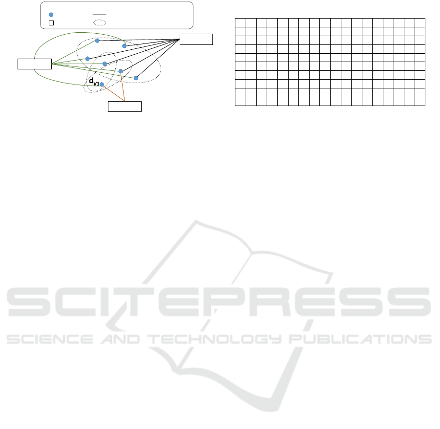
Figure 1: Use Case: A Location-based OSN service.

ters across the globe. Similar is the case for OSNs

as well. (2) Moving ahead, since the users of OSN

services like Facebook may register check-ins at vari-

ous locations across the world, not only the data-items

but also the source locations of data requests are geo-

graphically distributed.

Motivated by the above discussions, the problem

of data placement for data-intensive services in data-

centers that are distributed geographically across the

world is the topic of research detailed in this pa-

per. The use case under investigation is a location-

based OSN service as portrayed in Fig 1. A sample

Facebook social network is represented using a graph

where each vertex corresponds to a user and undi-

rected edges between two vertices represent friend-

ship. In this network, users {v

} are friends of the

user v

. Similarly {v

} are friends of v

. Addi-

tionally, the list of all the friends of every user is also

portrayed in the table presented right above the social

network. Each user can register a check-in, which is

denoted by her user-id assigned to a datacenter near-

est to her check-in location. In Fig. 1, the user v

has registered two check-ins, at datacenters located

in Virginia and Tokyo respectively, while user v

has

checked-in at Frankfurt. Moreover, each user check-

in requires data-items corresponding to all her friends,

which constitutes the data request pattern triggered

by this check-in. For example, a check-in by user v

in Sydney would trigger a data request requiring the

data-items corresponding to her friends {v

} to be

transferred to that location.

While data placement has been studied exten-

sively (Golab et al., 2014; Yuan et al., 2010; Ebrahimi

et al., 2015; Jiao et al., 2014), literature on geo-

distributed data-intensive services is relatively scarce

(Yu and Pan, 2017). Any successful solution to this

problem should provide two capabilities, namely –

capturing and improving (1) data-item – data-item

associations; and (2) data-item – datacenter associa-

tions. State-of-the-art methods proposed in (Nishtala

et al., 2013) and (Agarwal et al., 2010) are capable

of improving data-item – data-item, and data-item –

datacenter associations respectively, however, these

methods cannot jointly handle both aspects. To jointly

incorporate both aspects, (Yu and Pan, 2015; Yu

and Pan, 2017) recently proposed a multi-objective

data placement algorithm using hypergraphs. Hy-

pergraphs offer a powerful representation by present-

ing a natural way of capturing multi-way relation-

ships. Similar to graph partitioning however, hyper-

graph partitioning is NP-Hard. To this end, the au-

thors use heuristic partitioning algorithms available in

a publicly available tool – PaToH (Catalyurek, 2011),

to efﬁciently partition large hypergraphs. However,

as shown in Sec. 6, PaToH lacks scalability under cer-

tain scenarios while also suffering in terms of efﬁcacy.

To bridge this gap, in this paper, we propose a novel

scalable method for data placement through Spectral

Clustering on Hypergraphs.

Owing to their strong mathematical properties

spectral methods have been shown to be promising

in a plethora of areas of machine learning with semi-

nal research by (Shi and Malik, 2000; Spielmat, 1996;

Meila and Shi, 2001; Ng et al., 2001). Despite the ad-

vantages offered by spectral methods: superior efﬁ-

cacy, strong mathematical properties etc., they are not

usually efﬁcient and scalable on large scale data. We

mitigate the issue of lack of scalability by proposing

an approximate spectral clustering algorithm, thereby

bringing the power of spectral methods to perform ef-

fective hypergraph clustering. To summarize, the key

contributions of this work are as follows.

• We study the data placement problem in a chal-

lenging and close to real-world setting of data-

intensive services in geo-distributed datacenters

(Sec. 3), where traditional methods of hash based

partitioning that are prominent in systems like

Hadoop and Spark do not perform well.

• We propose a novel scalable algorithm to solve

the data placement problem for geo-distributed

data-intensive services through Spectral Cluster-

ing on Hypergraphs (Sec. 4).

• Through extensive experiments on a real-world

trace-based social network dataset (Secs. 5 and 6),

we show that the proposed spectral clustering al-

gorithm is scalable, and provides a speed-up of

up to 10 times over the state-of-the-art hyper-

graph partitioning method while portraying sim-

ilar (or in some cases even better) efﬁcacy on sev-

eral evaluation metrics.

2 RELATED WORK

The data placement problem has been studied ex-

tensively in the literature spanning a wide-variety of

CLOSER 2018 - 8th International Conference on Cloud Computing and Services Science

498

research areas, both from the perspective of execu-

tion environments: ranging from distributed systems

(Chervenak et al., 2007; Golab et al., 2014) to cloud

computing environments (Yuan et al., 2010; Li et al.,

2017; Ebrahimi et al., 2015; Liu and Datta, 2011); ap-

plication areas: online social network services (Jiao

et al., 2014; Han et al., 2017), location aware data

placement for geo-distributed cloud services (Yu and

Pan, 2017; Zhang et al., 2016; Yu and Pan, 2015; Yu

and Pan, 2016; Agarwal et al., 2010), and many more.

Here, we provide an overview the existing works that

overlap with our problem.

Research on data placement in geo-distributed

clouds has increasingly gained popularity over the

years. Owing to multiple niche challenges as dis-

cussed in Sec. 1, specialized solutions have been de-

vised to solve this problem. The biggest challenge

for data placement algorithms in such scenarios is that

data migrations from one location to another is signif-

icantly more expensive and problematic when com-

pared to other real-world scenarios like grids, clusters,

or private clouds where distance between data-centers

is not signiﬁcant.

(Agarwal et al., 2010) proposed a system: Volley,

to perform automatic data placement in geographi-

cally distributed datacenters. The proposed system

possesses the capability to capture data-item – dat-

acenter associations, however, it lacked the capabil-

ity for handling data-item – data-item associations.

(Jiao et al., 2014) formulates a multi-objective so-

cial network aware optimization problem that per-

forms data placement by building a model frame-

work, which takes multiple objectives into consider-

ation. (Han et al., 2017) introduce an adaptive data

placement algorithm for social network services in a

multicloud environment, which adapts to the chang-

ing data trafﬁc for performing intelligent data migra-

tion decisions. (Rochman et al., 2013) have focused

on placing data in a distributed environment to en-

sure that a large fraction of region speciﬁc requests

are served at a lower cost. In (Huguenin et al., 2012),

a user generated content (UGC) dataset (with more

than 650000 YouTube videos) is used to show the cor-

relation between the content locality and geographic

locality. (Zhang et al., 2016) propose an integer pro-

gramming based data placement algorithm capable of

minimizing the data communication cost while honor-

ing the storage capacity of geo-distributed datacenters

as well.

Researchers have also focused on the design of

specialized replication strategies for geo-distributed

services. (Kayaaslan et al., 2013) have proposed a

document replication framework to deal with the scal-

ability issues. In this replication framework, docu-

Table 1: Summary of notations used.

Item Deﬁnition

V The set of users in the social network V = {v

,..., v

E The set of edges in the social network ∀e = (v

) ∈ E.

Adj(v) The set of friends of the user v | v ∈ V.

D The set of data-items D = {d

,..., d

L The set of datacenters and their locations L = {L

,..., L

R The set of request patterns R = {R

,..., R

C The set of user check-ins C = {C

= (R

) | ∃R

∈ R , L

∈ L}.

Π The hypergraph incidence matrix.

The hyperedge weight matrix.

Φ The desired datacenter storage distribution.

P (D) A partition on the set of data-items D.

Γ(L

) Cost (per unit) of outgoing trafﬁc from datacenter L

κ(L

) Inter datacenter latency (directed) between L

and L

S(L

) Storage cost (per unit) of datacenter L

N (R

) Average number of datacenters accessed by request R

ments are replicated on datacenters based on region

speciﬁc user interests. (Shankaranarayanan et al.,

2014) propose replication strategies for a class of

cloud storage systems denoted as quorum-based sys-

tems (viz. Cassandra, Dynamo) capable of solv-

ing the data placement problem cognizant of var-

ious location-aware metrics like location of geo-

distributed datacenters, inter-datacenter communica-

tion costs etc.

(Golab et al., 2014) prove the reduction of data

placement problem to the well known graph parti-

tioning problem and propose an integer linear pro-

gramming solution. The authors also propose two

scalable heuristics to reduce the data communication

cost for data-intensive scientiﬁc workﬂows and join-

intensive queries in distributed systems. In (Qua-

mar et al., 2013), the authors study the problem of

OLTP workloads in cloud computing environments,

and propose a scalable workload aware data partition-

ing and data placement approach called SWORD to

reduce the partitioning overhead. SWORD is pro-

posed as a two phase approach: in the ﬁrst phase a

workload is modeled as a hypergraph which is further

compressed by using hash partitioning, and later the

compressed hypergraph is partitioned to get the place-

ment output. Hypergraph based partitioning solutions

(Catalyurek et al., 2007) have also been used in grid

and distributed computing environments previously.

Recently, (Yu and Pan, 2015; Yu and Pan, 2016;

Yu and Pan, 2017) propose data placement strategies

using hypergraph modeling and publicly available

partitioning heuristics (Catalyurek, 2011) for data-

intensive services, which constitutes the current state-

of-the-art for location-aware data placement in geo-

distributed clouds. The research presented in this pa-

per proposes a novel hypergraph partitioning scheme

using spectral clustering and enjoys strong mathemat-

ical properties and improved efﬁcacy when compared

to the competing techniques. Moreover, it enjoys su-

perior efﬁciency and scalability by employing low-

rank matrix approximations while retaining the same

efﬁcacy as portrayed by the state-of-the-art.

Scalable Data Placement of Data-intensive Services in Geo-distributed Clouds

499

Virginia

Frankfurt

California

Tokyo

Sydney

Datacenters

Data)Request)Patterns

Data)item

Data)Request)pattern

Data)Request)- Datacenter)Edge

Figure 2: Mapping of different requests to geo-distributed

datacenters.

3 PROBLEM STATEMENT

In this section, we formally deﬁne the data placement

problem for data-intensive services in geo-distributed

datacenters. Table 1 summarizes the notations used in

the rest of the paper.

A location based online social network (Fig. 1)

is represented using a graph G(V, E), where V rep-

resents the set of users, and E represents the set of

edges (denoting friendship) between any two users of

the social network. The set D contains n data-items

corresponding to each user v ∈ V of the social net-

work. Each user v ∈ V can register a check-in, where

a check-in is a tuple C

= (R

) ∈ C composed of

a data request pattern R

∈ R and a datacenter loca-

tion L

∈ L. Each data request pattern R

is com-

prised of a set of data-items D ⊆ D requested by a

user v ∈ V . As discussed in Sec. 1, considering the lo-

cation based social networks use-case, a data request

pattern R

belonging to a check-in C

registered by

a user v would comprise the data-items correspond-

ing to all the friends of v, i.e. R

= {d

| u ∈ Adj(v)}.

Moving ahead, L

∈ L represents the location of a dat-

acenter capable of serving user requests. The location

of a check-in C

is decided as the datacenter location

closest (in distance) to the actual physical location

of the user check-in. In other words, the check-in C

signiﬁes a request for data-items contained in R

trig-

gered from the datacenter located at L

Next, we discuss the basic concepts described

above in the context of the location based online so-

cial networks use-case presented in Sec. 1. Fig. 2

builds upon the example portrayed in Fig. 1 to show-

case the data request patterns corresponding to the

check-ins registered by users v

, and v

. Let us

denote the data request patterns as R

, and R

respectively, where R

= {d

}, and R

= {d

}. Let us also la-

bel the datacenter locations as L

= Virginia,L

Cali f ornia,L

= Frank f urt,L

= Sydney, and L

Tokyo. Recall that the user v

registered two check-

ins: one in Virginia and the other in Tokyo. Simi-

larly, v

registered a check-in in Frankfurt, while v

checked-in in Tokyo. Thus, in total there are four

check-ins: two (C

and C

) for the user v

, and one

each (C

and C

respectively) for users v

and v

where C

= (R

), C

= (R

), C

= (R

), and

= (R

Having deﬁned the basic concepts and their nota-

tions, we formally deﬁne the problem as:

Problem. Given a set of n data-items D, m user

check-ins C

= (R

) ∈ C , each comprising a data

request pattern R

being originated from a datacen-

ter located at L

, a set of l datacenters with loca-

tions in L, with the per unit cost of outgoing traf-

ﬁc from each datacenter ∀L

∈ L,Γ(L

), the per unit

storage cost of each datacenter ∀L

∈ L,S (L

), the

inter datacenter latency (directed) for each pair of

datacenters ∀L

∈ L,κ(L

), and the average

number of datacenters accessed by the data-items re-

quested in each request pattern R

being N (R

), per-

form data placement to minimize the optimization ob-

jective O, which is deﬁned as the weighted average of

Γ(·),κ(·,·),S(·), and N (·).

4 SPECTRAL CLUSTERING ON

HYPERGRAPHS

To effectively solve the data placement problem, we

propose a technique as outlined in Algorithm 1. Given

the set of data items D, and the set of user check-ins C

comprising the set of data request patterns R and their

locations L, we ﬁrst construct a hypergraph. As dis-

cussed in Sec. 1, hypergraphs provide the capability

to capture multi-way relationships, thereby facilitat-

ing modeling of data-item – data-item and data-item –

datacenter location associations. With the hypergraph

incidence matrix Π constructed, next, we partition the

set of data-items D into l parts corresponding to the L

datacenters according to the desired storage distribu-

tion Φ, using the proposed scalable spectral clustering

algorithm. Fig. 3 portrays the overall scheme of our

method.

We next explain each of the fundamental steps in

detail.

Workload

Set+of+User+

Check-ins+

($)

Hypergraph+

Modelling

Hypergraph+

Incidence+

Matrix+(")

Spectral+

Clustering

Data+

Placement+

Output

Figure 3: Overview of our Approach.

CLOSER 2018 - 8th International Conference on Cloud Computing and Services Science

500

4.1 Hypergraph Modeling

Continuing our discussion in Sec. 1, hypergraphs pro-

vide the ideal representation to solve the data place-

ment problem in geo-distributed datacenters owing

to their capability of capturing multi-way relation-

ships. A hypergraph H(V

) is a more sophis-

ticated graph construct and a generalization over a

graph G(V,E), where (hyper)edges are capable of

capturing relationships between several vertices as

opposed to just a pair of vertices in graphs. This abil-

ity of hyperedges to capture higher order relationships

between data points facilitates the hypergraph model

to manage both data-item – data-item and data-item –

datacenter locations associations.

Algorithm 1: Data Placement Algorithm.

Input: D, C , R , L, G(V,E), Φ

Output: Partitioning of the set of data-items P (D) into l

datacenters

1: (Π, W

) ← ConstructHypergraph(D,C , G(V,E))

2: P (D) ← SpectralClustering(Π, W

,l, Φ)

3: return P (D)

In the context of our problem statement, every

user check-in C

∈ C consists of a datacenter loca-

tion L

∈ L and a data request pattern R

∈ R . Note

that for a check-in by a user v, R

is a set of data-

items corresponding to all the friends of v, i.e. Adj(v),

as portrayed by the social network G(V,E). Since a

data request pattern involves data-items correspond-

ing to multiple vertices of G(V,E), hyperedges pro-

vide a better way to model data-item – data-item as-

sociations by linking/connecting multiple data-items

via the same hyperedge. Additionally, hyperedges

also facilitate modeling of data-item – datacenter lo-

cation associations by connecting a data-item with a

datacenter location when a data-item d

is requested

from a datacenter location L

The hypergraph vertex set V

comprises of all the

data-items D and the datacenter locations L. Thus,

the number of vertices in the hypergraph are |V

| =

= n + l. Formally,

= D ∪ L (1)

Let R

= {∀d ∈ R

,∀L

∈ L|∃C

= (R

) ∈

C ,R

d j

} denote the set of edges connecting data-items

with datacenter locations corresponding to all the data

request patterns R

∈ R triggered by user check-ins

∈ C at datacenter locations L

∈ L. The hyper-

graph edge set E

consists of hyperedges correspond-

ing to all the data request patterns R and all the data-

item – datacenter location edges R

. Thus, the num-

ber of hyperedges in the hypergraph are |E

| = m

r + nl. Formally,

= R ∪ R

(2)

Fig. 4a portrays the hypergraph representation of

the data-items and request patterns as presented in

Fig. 2. The data-items {d

,. ..,d

} and the dat-

acenter locations {L

} constitute the hyper-

graph vertex set. The hyperedges corresponding to

the data request patterns {R

} are labeled as

he1,he2, he3 respectively and are denoted using a

dashed ellipse, while the hyperedges connecting each

data-item – datacenter location pair are labeled as

he4,. ..,he17. Since v

are friends

of v

, the data-items d

,. ..,d

belonging to the

request pattern R

are connected by the hyperedge

he1. Similarly, since v

is a friend of v

, who reg-

istered two check-ins: one at Virginia (L

) and the

other at Tokyo (L

), the hyperedge he4 = (d

) and

he10 = (d

) represents the relationship between

the data-item d

and the datacenter locations where

it was requested, namely – Virginia (L

) and Tokyo

). Fig. 4b portrays the incidence matrix Π corre-

sponding to the hypergraph H presented in Fig. 4a.

As can be seen, the rows of this matrix are the ver-

tex set of the hypergraph, while the columns are the

hyperedges. Moreover, if a vertex participates in a hy-

peredge then the row corresponding to it contains a 1

in the column corresponding to that hyperedge, and

0 otherwise. Since the hyperedge he1 (corresponding

to the data request pattern R

) connects the data-items

,. ..,d

the entries in Π corresponding to them are

ﬁlled with 1 while all other entries are 0.

4.1.1 Calculating Hyperedge Weights

Having constructed the hypergraph H(V

) and

discussed its representation using a hypergraph in-

cidence matrix Π, we next discuss ways to assign

weights to hyperedges. There are two major types

of hyperedges constructed in the representation dis-

cussed above: (1) Data request pattern hyperedges,

and (2) Data-item – Datacenter hyperedges, and both

of them capture different properties required by a data

placement algorithm in geo-distributed datacenters.

The weight of a data request pattern hyperedge W

is set using the request rate of that pattern, which is

deﬁned as the number of times a data request pattern

is triggered by a user check-in. The weight W

fa-

cilitates prioritization of data-items that are usually

requested together, to be placed together by the data

placement algorithm, thereby helping optimize (min-

imize) N (R

): the average number of datacenters ac-

cessed by a data request pattern R

. On the other hand,

the weights (W

) corresponding to data-

item – datacenter hyperedges (R

) facilitate mini-

mization of inter datacenter latency κ(L

), storage

cost S (L

), and cost of outgoing trafﬁc Γ(L

) respec-

Scalable Data Placement of Data-intensive Services in Geo-distributed Clouds

501

"%&'%(%)

*+,-+

.&)(,/0&1

Vertex&Set

Data&item

Datacenter

Hyperedge Set

Data&item&– Datacenter&edge

Data&Request&pattern&edge

789:6

789:4

;

789:;

9:#8= 9:>

9:6?8= 9:63

9:6@

9:62

(a) Hypergraph Representation

0 1 1 0 0 0 0 0 0 0 1 0 0 0 0 0 1 0

1 0 1 1 0 0 0 0 0 1 0 0 0 0 0 0 0 0

1 1 0 0 1 0 0 0 0 0 0 1 0 0 0 0 0 1

1 0 0 0 0 1 0 0 0 0 0 0 1 0 0 0 0 0

1 0 0 0 0 0 1 0 0 0 0 0 0 1 0 0 0 0

1 0 0 0 0 0 0 1 0 0 0 0 0 0 1 0 0 0

1 0 0 0 0 0 0 0 1 0 0 0 0 0 0 1 0 0

0 0 0 1 1 1 1 1 1 0 0 0 0 0 0 0 0 0

0 0 0 0 0 0 0 0 0 0 0 0 0 0 0 0 1 1

0 0 0 0 0 0 0 0 0 1 1 1 1 1 1 1 0 0

he1

he2% he3% he4%

he5% he6% he7

he8%

he9

he10%

he11%he12%

he13%

he14%

he15%

he16%he17%

Hypergraph%Incidence%Matrix%(")

he18%

(b) Hypergraph Incidence Matrix

Figure 4: Modeling the data request patterns triggered by user check-ins as a Hypergraph.

tively, by giving priority to placing data-items at data-

center locations from where they have been requested

more frequently.

The resultant hyperedge weight matrix W

of Π is

a diagonal matrix of size m

× m

, which is deﬁned as

the weighted sum of W

, W

, and W

. Math-

ematically,

= W · (W

). (3)

where, W is the weight vector for deciding the priori-

ties of the previously discussed hyperedge weighting

strategies.

4.2 Spectral Clustering

Spectral methods have been shown to be promising

in a plethora of machine learning research areas: im-

age segmentation (Shi and Malik, 2000; Meila and

Shi, 2001), data clustering (Ng et al., 2001), web

search (Gibson et al., 1998), and information retrieval

(Deerwester et al., 1990). The power of these algo-

rithms is that they possess both sound mathematical

properties and strong empirical prowess. They are

named spectral algorithms as they use the information

manifested within the spectra (both eigen-values and

eigen-vectors) of a similarity/afﬁnity matrix. More

fundamentally, for a graph G represented using a sim-

ilarity matrix containing node-node similarities, these

methods use the spectra of the graph laplacian to un-

derstand the intrinsic data properties like structure,

connectivity etc. Interestingly, the laplacian for hy-

pergraph was derived in (Zhou et al., 2006), where it

is shown to be analogous to the simple graph lapla-

cian. This result facilitates application of spectral

methods on hypergraphs.

Having discussed about the importance of spec-

tral methods, we next describe the proposed algo-

rithm for performing spectral clustering on hyper-

graphs. The ﬁrst step in spectral clustering on hyper-

graphs is to construct the hypergraph laplacian ma-

trix L

. The output of the hypergraph construction

step is a n

× m

dimensional hypergraph incidence

matrix Π and a m

× m

dimensional diagonal hyper-

edge weight matrix W

. As discussed previously, the

hypergraph incidence matrix Π = [he

,he

,. ..,he

]

possesses m

hyperedges, where each hyperedge he

[he

1,i

,he

2,i

,. ..,he

] is a n

-dimensional binary vec-

tor. The entry he

j,i

= 1 indicates that the j

vertex

in the hypergraph vertex set is participating in the i

hyperedge, while he

j,i

= 0 indicates otherwise. With

this, the hypergraph laplacian L

is deﬁned as:

= I − (D

−1/2

ΠW

−1

−1/2

) (4)

where, I is a n

× n

identity matrix;

is a n

× n

diagonal vertex degree matrix deﬁned

as D

= diag(

∑

Π);

is a m

×m

diagonal hyperedge degree matrix de-

ﬁned as D

= diag(

∑

);

is a m

× m

diagonal hyperedge weight ma-

trix deﬁned as W

= diag([W

,. ..,W

]), and

,. ..,W

are calculated as described in Eq. 3. Thus,

becomes a n

× n

matrix.

The next step is to perform eigen-decomposition

of the hypergraph laplacian matrix L

, in order

to identify its spectra: the eigen-values and eigen-

vectors. The eigen-decomposition of L

is written

as:

= UΛV (5)

where,

U = [u

,. ..,u

] is a n

× n

matrix formed by the

eigen-vectors of L

;

Λ = diag(λ

,. ..,λ

) is a diagonal n

× n

matrix

formed by the eigen-values of L

and,

V = U

since L

is a square symmetric matrix.

The eigen-vectors U and eigen-values Λ collec-

tively deﬁne the spectra for the hypergraph laplacian

As discussed in Sec. 1, despite their strong theo-

retical and mathematical properties, spectral methods

are usually not scalable. This is mainly due to the

CLOSER 2018 - 8th International Conference on Cloud Computing and Services Science

502

complex operation of performing a full eigen decom-

position of a large matrix, which is cubic O(n

) in

the dimensionality of L

in the worst case. Having

said that, it is shown in the literature (Zhou et al.,

2006) that it is not required to use all the eigen-

vectors and thus, in practice one may work with just

a small fraction of n

. To this end, we work with a

low-rank approximation of L

, thereby restricting the

eigen decomposition to just calculate the 100 small-

est eigen vectors of L

. To scale this operation fur-

ther, we employ the use of randomized methods to

perform approximate partial matrix decompositions

(Halko et al., 2011), which again works very well in

practice without any signiﬁcant loss in accuracy. As

will be explained later in Sec. 6, these randomized

methods facilitate the proposed spectral clustering al-

gorithm to achieve superior efﬁciency and scalability,

without any loss in the efﬁcacy.

The last step involves performing k-means clus-

tering on the eigen-vectors U of the hypergraph lapla-

cian matrix L

. Since we know the number of dat-

acenter locations a priori, which is l = |L|, we par-

tition U into l clusters. This operation partitions

the set of data-items D into l different sets, thereby

forming P (D), which is used as the placement de-

cision recommended by the proposed data placement

algorithm. The clustering approach used here is not

a vanilla k-means, rather it includes multiple exten-

sions. First, to ensure load balancing we modify

the objective function of k-means to honor the de-

sired storage distribution Φ, which provides informa-

tion about the expected capacity of each datacenter

location. Second, we employ the use of k-means++

initialization as proposed in (Arthur and Vassilvitskii,

2007) and parallelization to scale-up the clustering al-

gorithm to very large datasets.

The three step process: (1) Hypergraph Laplacian

construction, (2) Eigen decomposition of the hyper-

graph laplacian, and (3) k-means clustering on the

eigen-vectors, with added extensions and modiﬁca-

tions constitutes the proposed scalable spectral clus-

tering algorithm.

Note that the approach discussed above is capable

of solving the data placement problem without con-

sidering the possibility of replicas. Since replication

may be important in real-world settings for ensuring

fault-tolerance and load-balancing, we brieﬂy discuss

an extension to allow for the scenarios with replica-

tion as well. To this end, we use the proposed data

placement algorithm to get a placement without repli-

cation, however, we change the capacity of each dat-

acenter from s

to s

/r, where r is the desired repli-

cation factor. We then execute the same algorithm r

times on different permutations of the set of datacen-

ters L. This allows the same data-item to be stored (in

the expected sense) on r datacenters, thereby meeting

the desired replication factor. With this, the proposed

algorithm is extended to handle scenarios where repli-

cation is allowed as well. For the sake of brevity, we

keep this discussion around extensions to scenarios

with replication short. A detailed analysis and eval-

uation of various replication strategies will constitute

as future work.

5 EVALUATION SETUP

5.1 Geo-distributed Datacenters

To simulate a real-world geo-distributed cloud envi-

ronment, we employ the use of l = 9 geo-distributed

datacenters based on the regions provided by AWS

global infrastructure (aws, 2017). Note that the AWS

infrastructure evolves continuously and for the sake

of standardization and reproducible comparison with

previous work (Yu and Pan, 2015), we only chose

the 9 oldest and prominent regions, namely: Vir-

ginia, California, Oregon, Ireland, Frankfurt, Singa-

pore, Tokyo, Sydney, and Sao Paulo, for our exper-

imental setup. Our experimental setup closely mir-

rors the actual AWS setup, as the costs involved for

storage and outgoing trafﬁc as indicated in Table 2a

are as advertised by Amazon. Moreover, the inter-

datacenter latencies(aws, 2016) are also measured by

the packet transfer latency between the chosen regions

using the Linux ping command. Table 2b presents

the average inter-datacenter latency values (in ms) be-

tween the 9 chosen datacenter regions. It is evident

from the values portrayed in Table 2 that the proper-

ties exhibited by datacenters vary signiﬁcantly with

the region, and hence, any data placement strategy

should incorporate this knowledge while performing

placement decisions.

5.2 Data

The dataset used in our experiments is a trace of

a location-based online social network – Gowalla

available publicly from the SNAP (sna, 2017) repos-

itory. The Gowalla dataset has been used extensively

(Yu and Pan, 2015; Yu and Pan, 2017) for data place-

ment research in geo-distributed cloud services. The

social network contains 196591 vertices and 950327

edges. The vertices are the users in the social network,

while the edges represent friend relationship between

http://snap.stanford.edu/data/loc-gowalla.html

Scalable Data Placement of Data-intensive Services in Geo-distributed Clouds

503

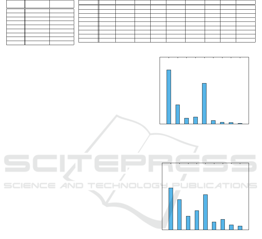
Table 2: (a) Trafﬁc and Storage Costs, and (b) Inter Datacenter Latency (in ms) based on Geo-distributed Amazon Clouds.

(a) Costs (in $)

Region

Storage Outgoing

($/GB-month) Trafﬁc ($/GB)

Virginia 0.023 0.02

California 0.026 0.02

Oregon 0.023 0.02

Ireland 0.023 0.02

Frankfurt 0.025 0.02

Singapore 0.025 0.02

Tokyo 0.025 0.09

Sydney 0.025 0.14

Sao Paulo 0.041 0.16

(b) Latency (in ms)

Region Virginia California Oregon Ireland Frankfurt Singapore Tokyo Sydney Sao-Paulo

Virginia 0.0 72.738 86.981 80.546 88.657 216.719 145.255 229.972 119.531

California 71.632 0.0 19.464 153.202 166.609 174.010 102.504 157.463 192.670

Oregon 88.683 19.204 0.0 136.979 159.523 161.367 89.095 162.175 182.716

Ireland 80.524 153.220 136.976 0.0 19.560 239.023 212.388 309.562 191.292

Frankfurt 88.624 166.590 159.542 19.533 0.0 325.934 236.537 323.483 194.905

Singapore 216.680 173.946 161.423 238.130 325.918 0.0 73.807 175.328 328.080

Tokyo 145.261 102.523 89.157 212.388 236.558 73.785 0.0 103.907 256.763

Sydney 229.748 157.843 161.932 309.562 323.152 175.355 103.900 0.0 322.494

Sao Paulo 119.542 192.700 181.665 191.559 194.900 327.924 256.665 322.523 0.0

two users. The trace provides 6442890 user check-

ins logged over the period of February, 2009 to Octo-

ber, 2010. As described in Sec. 3, each user check-in

consists of a data request pattern and a location. In

continuation to our discussions in Sections 1 and 3,

a request (indicated by a check-in) by a user v would

involve pulling the data of all his/her friends. Thus,

the data request pattern corresponding to a check-in

by a user v is the set of data-items corresponding to

all the friends of v, i.e. Adj(v). The location ﬁeld of

a user check-in are the GPS coordinates of the place

from where the check-in was triggered. These GPS

coordinates were mapped to the closest (in terms of

distance) datacenter region to identify the source lo-

cation of a data request pattern, and can thus, be one

of the 9 datacenter regions as described in Sec. 5.1.

With this pre-processing, we obtain a use-case sce-

nario consisting of 196591 data-items and 102314

data request patterns.

Moving ahead, we present certain dataset statis-

tics. Fig. 5 portrays the distribution of user check-ins

across the 9 datacenter regions discussed above. It is

evident that Virginia and Frankfurt register the high-

est (≈ 40%) and the second highest (≈ 30%) number

of user check-ins. On the other hand, Tokyo, Syd-

ney, and SaoPaulo get the fewest (≈ 10% combined)

number of user check-ins. This clearly shows a huge

disparity in the check-in distribution. Based on the

user check-in distribution, we extract the storage size

distribution Φ of the datacenter regions, which is de-

pendent upon both the number of check-ins registered

in a region and the size of data request pattern trig-

gered by the check-in. As is clear from Fig. 6, the

desired storage distribution portrays a similar trend

as that of the check-in distribution. Note that this

storage distribution Φ also serves as an input to the

data placement algorithm, thereby facilitating load-

balancing among the 9 datacenter regions. More fun-

damentally, the load-balancing factor is calculated as

the expected storage size at each datacenter region us-

ing the storage distribution Φ.

0.1

0.2

0.3

0.4

0.5

Virginia

California

Oregon

Ireland

Frankfurt

Singapore

Tokyo

Sydney

SaoPaulo

Distribution of Check-ins

Figure 5: Distribution of user check-ins across geo-

distributed datacenters.

0.05

0.1

0.15

0.2

0.25

0.3

0.35

0.4

Virginia

California

Oregon

Ireland

Frankfurt

Singapore

Tokyo

Sydney

SaoPaulo

Distribution of Expected Storage Size

Figure 6: Distribution of expected datacenter storage size.

5.3 Algorithms

We compare the proposed data placement algorithm

using spectral clustering on hypergraphs for effective-

ness, efﬁciency, and scalability against a number of

baselines – Random and Nearest, and the state-of-the-

art hypergraph partitioning technique (Yu and Pan,

2015; Yu and Pan, 2017). All the algorithms were

implemented in C++. To perform hypergraph parti-

tioning for the technique proposed by (Yu and Pan,

2015) and reproduce their results we use the PaToH

(Catalyurek, 2011) toolkit. Next, we give brief de-

CLOSER 2018 - 8th International Conference on Cloud Computing and Services Science

504

scriptions of the compared techniques:

• Random: partitions the set of data-items D ran-

domly into |L| = l datacenters. To distribute the

data-items according to the datacenter storage size

distribution Φ, we ensure that random partitioning

samples data-items based on Φ thereby ensuring

load-balancing.

• Nearest: assigns each data-item to the datacen-

ter from where it has been requested the highest

number of times. Similar to random, to ensure

load-balancing this technique follows the datacen-

ter storage distribution Φ. Thus, once the dat-

center with the highest number of requests for a

particular data-item has reached its capacity, we

randomly choose a datacenter location capable of

serving new requests.

• Hypergraph Partitioning: is the data placement

algorithm proposed by (Yu and Pan, 2015; Yu and

Pan, 2017). After the hypergraph modeling step

discussed in Sec. 4, it uses the hypergraph parti-

tioning algorithms available in the PaToH toolkit.

The partitioning algorithms maintain the datacen-

ter storage size distribution Φ, thereby ensuring

load-balancing.

5.4 Parameters

As discussed in Sec. 4, different hyperedge weights

) facilitate optimization of dif-

ferent objectives. As stated in Eq. 3, a weight vector

W facilitates prioritization of these objectives based

on the assigned weights. In our study, we incorporate

the use of speciﬁc weight vector W settings: W

{100,1, 1,1}, W

: {1,100,1,1}, W

: {1,1,100,1},

and W

: {1,1,1,100}, which represent different pref-

erences or importance of the considered evaluation

metrics, such as, higher priority of collocating the as-

sociated data-items thereby minimizing the datacenter

span N (·), lower inter-datacenter trafﬁc Γ(·), lower

inter-datacenter latency κ(·), and lower storage cost

S(·) respectively. Note that in all the weight-vector

settings, the value 100 is just used to indicate higher

relative importance of the corresponding metric. The

results portrayed are not dependent on the speciﬁc

value of 100, rather the weight-vectors can work with

any value as long as it is >> 1.

5.5 Evaluation Metrics

• Span (N (·)): of a data request pattern R

is de-

ﬁned as the average number of datacenters re-

quired to be accessed to fetch the data-items re-

quested in R

. Further, the span for the entire

workload is calculated as the average of the dat-

acenter spans of each request pattern R

∈ R .

• Trafﬁc (Γ(·)): The total trafﬁc cost of a data re-

quest pattern R

is deﬁned as the sum of outgoing

trafﬁc prices of the datacenters involved in out-

going requests for the data-items in R

. Further,

the trafﬁc cost of the entire workload is calculated

as the sum of trafﬁc costs of each request pattern

∈ R .

• Latency (κ(·)): The inter-datacenter latency of a

data request pattern R

is calculated as the sum

of access latencies required to fetch all the data-

items requested in R

from the datacenter where

they are placed to the datacenter from where the

request was triggered. Further, the latency of the

workload is calculated as the sum of the latencies

of each request pattern R

∈ R .

• Storage (S(·)): The sum of the total cost on stor-

ing all of the data-items corresponding to every

data request pattern R

∈ R in datacenters L pre-

scribed by the data placement algorithm.

• Balance: is calculated as the pearson’s correla-

tion coefﬁcient between the expected storage size

distribution Φ, and the actual storage size distri-

bution obtained after performing data placement.

If the value is close to 1, it means that the two dis-

tributions are highly similar, while they are dis-

similar if the value is close to −1.

• Objective. (Obj.): is deﬁned as the weighted sum

of the considered performance metrics, where the

weights are described using the weight vector W.

6 EVALUATION RESULTS

All the experiments were done using codes written in

C++ on an Intel(R) Xeon(R) E5-2698 28-core ma-

chine with 2.3 GHz CPU and 256 GB RAM run-

ning Linux Ubuntu 16.04. Owing to their non-

deterministic nature, results for the random and hy-

pergraph partitioning methods are averaged over 10

runs. Note that the results portrayed corresponding to

each evaluation metric (barring Balance) are normal-

ized in the scale of [0,1] by dividing each value by

the highest observed value in that particular metric.

Normalization ensures that all the values lie in a com-

mon range ([0,1]), thereby facilitating joint analysis

of all the considered evaluation metrics for all the al-

gorithms. Since the problem formulation in this study

is concerned with the minimization of the evaluation

metrics, the smaller the portrayed values the better the

performance is. Additionally, note that the results for

Scalable Data Placement of Data-intensive Services in Geo-distributed Clouds

505

0.2

0.4

0.6

0.8

Obj

Span

Traffic

Latency

Storage

Balance

Normalized Evaluation Metrics

Random

Nearest

Hyper

Spectral

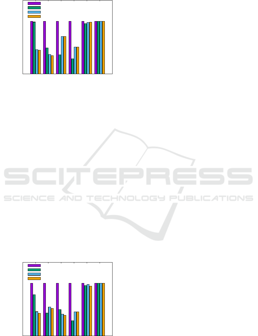
Figure 7: W

= {100, 1, 1,1}: Higher priority towards min-

imizing the datacenter span N (·).

the balance evaluation metric are close to 1 for all the

techniques considered in this study. This is because

every technique possesses the capability to honor the

desired storage size distribution Φ.

Fig. 7 presents the results corresponding to the

weight-vector setting W

, where minimizing the data-

center span holds the highest priority in the optimiza-

tion objective. It is evident that both, the proposed

spectral clustering algorithm (Spectral), and the state-

of-the-art hypergraph partitioning algorithm (Hyper)

achieve a low value on the overall optimization ob-

jective (Obj), while being signiﬁcantly better than the

random and nearest methods. This is because of their

capability to preferentially minimize the datacenter

span, which possesses the highest priority in the opti-

mization under W

. Note that Nearest outperforms

both Hyper and Spectral on the trafﬁc and latency

metrics, as they have lower weights in the optimiza-

tion objective under W

. However, both Spectral and

Hyper are still signiﬁcantly better than the Random

method.

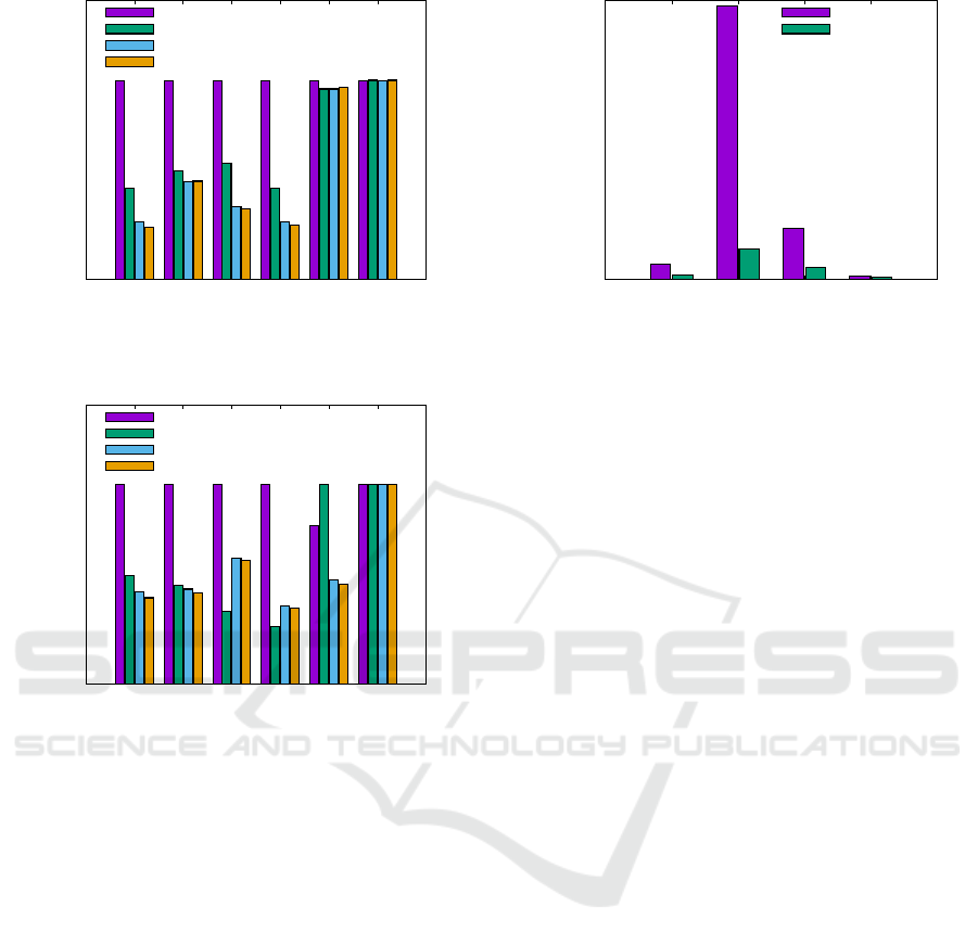
A similar behavior is observed in Figs. 8, 9, and

10 corresponding to the other three weight vector set-

0.2

0.4

0.6

0.8

Obj

Span

Traffic

Latency

Storage

Balance

Normalized Evaluation Metrics

Random

Nearest

Hyper

Spectral

Figure 8: W

= {1, 100, 1,1}: Higher priority towards min-

imizing the inter-datacenter trafﬁc Γ(·).

tings W

, W

, and W

respectively. Both Spectral

and Hyper outperform the other methods signiﬁcantly

on the overall optimization (Obj), while also being

signiﬁcantly better on the corresponding evaluation

metric that the weight-vector setting is tuned to op-

timize. More fundamentally, in addition to being bet-

ter on Obj., both Spectral and Hyper outperform the

other methods in minimizing inter-datacenter trafﬁc

cost Γ(·), inter-datacenter latency κ(·), and storage

cost S(·), when a higher preference is given to these

metrics under the weight-vector settings W

, W

, and

respectively.

The main limitation of Nearest is that it tries to

assign each data-item to a datacenter with the high-

est number of accesses to that data-item, thereby aim-

ing to minimize (on an average) the geographical dis-

tance between the data-item and the source location

of the data request oblivious to the fact that the ac-

tual trafﬁc or storage costs might not be proportional

to the distance. The main advantage of both Spectral

and Hyper over Nearest is that owing to their higher-

order modeling capabilities they are capable of better

addressing multi-objective optimizations, and possess

the capability to adapt their performance based on dif-

ferent weight-vector settings. This is evident from the

results portrayed in Figs. 7– 10. To further empha-

size on the capability to adapt the optimization based

on different weight-vector settings, we discuss the re-

sults portrayed in Fig. 10. It is clear that according

to W

, the optimization objective gives more prefer-

ence towards minimizing the storage cost. Note that

storage cost and other parameters like inter-datacenter

trafﬁc and latency might be inversely related to each

other, i.e., a lower storage cost might lead to higher

latencies or trafﬁc cost. This behavior is also evident

from Fig. 10, where both Spectral and Hyper achieve

lower storage costs, thereby also achieving better per-

formance on Obj, however, suffer slightly on other

metrics. Thus, methods like Nearest would ﬁnd difﬁ-

culty in handling such cases, while both Spectral and

Hyper possess the capability to adapt the optimization

based on the weight-vector.

Figs. 7– 10 show that the performance of both

Spectral and Hyper are quite similar on the evaluated

metrics. While Spectral is always marginally better in

efﬁcacy when compared to Hyper, the major advan-

tage of Spectral over Hyper comes from its capabil-

ity to scale gracefully and efﬁciently to large datasets.

It is intuitive that scalability is a paramount property

for any data placement algorithm, since the scale of

real-world social networks or for that matter any real-

world data-intensive services is humongous. Fig. 11

shows that Spectral is up to 10 times (≈ 3–4 times on

average) faster when compared to Hyper, while also

CLOSER 2018 - 8th International Conference on Cloud Computing and Services Science

506

0.2

0.4

0.6

0.8

Obj

Span

Traffic

Latency

Storage

Balance

Normalized Evaluation Metrics

Random

Nearest

Hyper

Spectral

Figure 9: W

= {1, 1, 100,1}: Higher priority towards min-

imizing the inter-datacenter latency κ(·).

0.2

0.4

0.6

0.8

Obj

Span

Traffic

Latency

Storage

Balance

Normalized Evaluation Metrics

Random

Nearest

Hyper

Spectral

Figure 10: W

= {1,1, 1,100}: Higher priority towards

minimizing the storage cost S(·).

being slightly better in all evaluated metrics for the

majority of the considered weight-vector settings.

In summary, through extensive experiments we

verify that the proposed spectral clustering algorithm

is efﬁcient, scalable, and effective. Although Spectral

is not always the best on every evaluated metric, it

serves to be the most effective technique in terms of

improving Obj, which is the main target of our multi-

objective optimization. Additionally, it possesses the

capability to adapt to the change in weight vector set-

tings W, which facilitates handling of a variety of

real-world scenarios as described by different weight

vectors.

7 CONCLUSIONS

In this paper, we have addressed the problem of

data placement of data-intensive services into geo-

distributed clouds. We identiﬁed the need for spe-

cialized methods to perform data placement for data-

intensive services, as contrary to MapReduce style

500

1000

1500

2000

2500

3000

Running Time (in secs.)

Hyper

Spectral

Figure 11: Efﬁciency of spectral clustering over hypergraph

partitioning.

workloads, these workloads require access to multi-

ple datasets within a single transaction, thus, render-

ing traditional methods of hash based partitioning in-

adequate. Consequently, we devised a scalable spec-

tral clustering algorithm for hypergraph partitioning,

thereby facilitating data placement. Experiments on

a real-world trace-based social network dataset por-

trayed the effectiveness, efﬁciency, and scalability of

the proposed algorithm. In the future, we would like

to design and develop a distributed version of our al-

gorithms and implement the entire system on state-of-

the-art big data technologies like Apache Spark. Ad-

ditionally, we would also like to include the notion of

replicas directly in the data placement problem for-

mulation.

ACKNOWLEDGEMENTS

This research is partly funded by the IWT SBO De-

CoMAdS project.

REFERENCES

(2015). How much data does X store? https://

techexpectations.org/2015/03/28/how-much-data-

does-x-store/.

(2016). Latency Between AWS Global Regions. http://

zhiguang.me/2016/05/10/latency-between-aws-

global-regions/.

(2017). AWS Global Infrastructure. https://aws.

amazon.com/about-aws/global-infrastructure/.

(2017). SNAP Datasets. https://snap.stanford.edu/data/.

(2017). The Exponential Growth of Data.

https://insidebigdata.com/2017/02/16/the-

exponential-growth-of-data/.

Agarwal, S., Dunagan, J., Jain, N., Saroiu, S., Wolman,

A., and Bhogan, H. (2010). Volley: Automated Data

Scalable Data Placement of Data-intensive Services in Geo-distributed Clouds

507

Placement for Geo-distributed Cloud Services. In

NSDI.

Arthur, D. and Vassilvitskii, S. (2007). k-means++: The

Advantages of Careful Seeding. In SODA, pages

1027–1035.

Catalyurek, U. V. (2011). PaToH (Partitioning Tool for

Hypergraphs). http://bmi.osu.edu/umit/PaToH/ man-

ual.pdf.

Catalyurek, U. V., Boman, E. G., Devine, K. D.,

Bozdag, D., Heaphy, R., and Riesen, L. A. (2007).

Hypergraph-based Dynamic Load Balancing for

Adaptive Scientiﬁc Computations. In IPDPS, pages

1–11.

Chervenak, A., Deelman, E., Livny, M., Su, M., Schuler,

R., Bharathi, S., Mehta, G., and Vahi, K. (2007). Data

Placement for Scientiﬁc Applications in Distributed

Environments. In GRID.

Deerwester, S. C., Ziff, D. A., and Waclena, K. (1990).

An Architecture for Full Text Retrieval Systems. In

DEXA, pages 22–29.

Ebrahimi, M., Mohan, A., Kashlev, A., and Lu, S. (2015).

BDAP: A Big Data Placement Strategy for Cloud-

Based Scientiﬁc Workﬂows. In BigDataService,

pages 105–114.

Gibson, D., Kleinberg, J., and Raghavan, P. (1998). Infer-

ring Web Communities from Link Topology. In HY-

PERTEXT, pages 225–234.

Golab, L., Hadjieleftheriou, M., Karloff, H., and Saha,

B. (2014). Distributed Data Placement to Minimize

Communication Costs via Graph Partitioning. In SS-

DBM, pages 1–12.

Halko, N., Martinsson, P., and Tropp, J. A. (2011). Find-

ing Structure with Randomness: Probabilistic Algo-

rithms for Constructing Approximate Matrix Decom-

positions. SIAM Review, 53(2):217–288.

Han, S., Kim, B., Han, J., K.Kim, and Song, J. (2017).

Adaptive Data Placement for Improving Performance

of Online Social Network Services in a Multicloud

Environment. In Scientiﬁc Programming, pages 1–17.

Huguenin, K., Kermarrec, A. M., Kloudas, K., and Ta

ıani,

F. (2012). Content and Geographical Locality in User-

generated Content Sharing Systems. In NOSSDAV,

pages 77–82.

Jiao, L., Li, J., Du, W., and Fu, X. (2014). Multi-objective

data placement for multi-cloud socially aware ser-

vices. In INFOCOM, pages 28–36.

Kayaaslan, E., Cambazoglu, B. B., and Aykanat, C. (2013).

Document Replication Strategies for Geographically

Distributed Web Search Engines. Inf. Process. Man-

age., 49(1):51–66.

Li, X., Zhang, L., Wu, Y., Liu, X., Zhu, E., Yi, H., Wang, F.,

Zhang, C., and Yang, Y. (2017). A Novel Workﬂow-

Level Data Placement Strategy for Data-Sharing Sci-

entiﬁc Cloud Workﬂows. IEEE TSC, PP(99):1–14.

Liu, X. and Datta, A. (2011). Towards Intelligent Data

Placement for Scientiﬁc Workﬂows in Collaborative

Cloud Environment. In IPDPSW, pages 1052–1061.

Meila, M. and Shi, J. (2001). Learning Segmentation by

Random Walks. In NIPS, pages 873–879.

Ng, A. Y., Jordan, M. I., and Weiss, Y. (2001). On Spec-

tral Clustering: Analysis and an Algorithm. In NIPS,

pages 849–856.

Nishtala, R., Fugal, H., Grimm, S., Kwiatkowski, M., Lee,

H., Li, H. C., McElroy, R., Paleczny, M., Peek, D.,

Saab, P., Stafford, D., Tung, T., and Venkataramani,

V. (2013). Scaling Memcache at Facebook. In NSDI,

pages 385–398.

Quamar, A., Kumar, K. A., and Deshpande, A. (2013).

SWORD: Scalable Workload-aware Data Placement

for Transactional Workloads. In EDBT, pages 430–

441.

Rochman, Y., Levy, H., and Brosh, E. (2013). Re-

source placement and assignment in distributed net-

work topologies. In INFOCOM, pages 1914–1922.

Shankaranarayanan, P. N., Sivakumar, A., Rao, S., and

Tawarmalani, M. (2014). Performance Sensitive

Replication in Geo-distributed Cloud Datastores. In

DSN, pages 240–251.

Shi, J. and Malik, J. (2000). Normalized Cuts and Image

Segmentation. PAMI, 22(8):888–905.

Spielmat, D. A. (1996). Spectral Partitioning Works: Planar

Graphs and Finite Element Meshes. In FOCS, pages

96–105.

Yu, B. and Pan, J. (2015). Location-aware associated data

placement for geo-distributed data-intensive applica-

tions. In 2015 IEEE Conference on Computer Com-

munications (INFOCOM), pages 603–611.

Yu, B. and Pan, J. (2016). Sketch-based data placement

among geo-distributed datacenters for cloud storages.

In INFOCOM, pages 1–9.

Yu, B. and Pan, J. (2017). A Framework of Hypergraph-

based Data Placement among Geo-distributed Data-

centers. IEEE TSC, PP(99):1–14.

Yuan, D., Yang, Y., Liu, X., and Chen, J. (2010). A

data placement strategy in scientiﬁc cloud workﬂows.

FGCS, 26(8):1200 – 1214.

Zhang, J., Chen, J., Luo, J., and Song, A. (2016). Efﬁ-

cient location-aware data placement for data-intensive

applications in geo-distributed scientiﬁc data centers.

Tsinghua Science and Technology, 21(5):471–481.

Zhou, D., Huang, J., and Sch

olkopf, B. (2006). Learn-

ing with Hypergraphs: Clustering, Classiﬁcation, and

Embedding. In NIPS, pages 1601–1608.

CLOSER 2018 - 8th International Conference on Cloud Computing and Services Science

508