
An Efficient Decentralized Multidimensional Data Index: A Proposal
Francesco Gargiulo
1
, Antonio Picariello
2
and Vincenzo Moscato
2
1
Italian Aerospace Research Centre, via Maiorise, Capua (CE), Italy
2
Department of Computing, University Federico II of Napoli, Napoli, Italy
Keywords: Distributed Index, Large Databases, Multidimensional Data Index, Decentralized K-Nearest Neighbour
Query.
Abstract: The main objective of this work is the proposal of a decentralized data structure storing a large amount of data
under the assumption that it is not possible or convenient to use a single workstation to host all data. The
index is distributed over a computer network and the performance of the search, insert, delete operations are
close to the traditional indices that use a single workstation. It is based on k-d trees and it is distributed across
a network of "peers", where each one hosts a part of the tree and uses message passing for communication
between peers. In particular, we propose a novel version of the k-nearest neighbour algorithm that starts the
query in a randomly chosen peer and terminates the query as soon as possible. Preliminary experiments have
demonstrated that in about 65% of cases it starts a query in a random peer that does not involve the peer
containing the root of the tree and in the 98% of cases it terminates the query in a peer that does not contain
the root of the tree.
1 INTRODUCTION
A multidimensional data index is a building block for
a variety of applications based on Linked open Data
(LOD) and Big Data. The LOD paradigm is gaining
increased attention in recent years and the size of the
phenomenon is considerable, we are talking about
hundreds of millions of information published in the
form of ”concepts” and of billions of connections
between these concepts (Abele, 2017). It is
reasonable to assume the proliferation of new
applications and new services that are able to take
advantage of this huge quantity of information.
Big Data is a term for data sets that are so large or
complex that traditional data processing software
applications are inadequate to deal with them. The
proposed index fits the requirements of LOD and Big
Data applications.
A decentralized multidimensional data index also is
suitable for sensor networks because they could
collect a very large amount of multidimensional data
(position, timestamp, temperature, pressure, etc.).
Often a subset of the nodes of the network can
manage a network connection, execute software and
store data, therefore the sensor network, through these
nodes, may implement itself the index.
Finally, a multidimensional data index is also
appropriate for text indexing. After the extraction of
a set of concepts C from the text (Basile, 2007) and
the introduction of a similarity measures d between
them, e.g. Resnik, Leacock & Chodorow, Wu &
Palmer (Corley, 2005), it is possible to build a metric
space (C, d). Well known mapping algorithms, such
as FastMap (Faloutsos, 1995) or MDS (Kruskal,
1978), calculate a mapping between this metric space
and a new vector space. The resulting points in this
vector space populates an instance of the
multidimensional data index as proposed in this work.
Range query and k-nearest on this data structure
query will return concepts that are also semantically
close concepts (with respect the similarity measure
chosen). A non-trivial example based on this
approach for a semantic driven requirements
consistency verification is (Gargiulo, 2015).
2 RESEARCH IDEAS AND
RESULTS
This section introduces the problem description and
our proposal to cope with it.
Gargiulo, F., Picariello, A. and Moscato, V.
An Efficient Decentralized Multidimensional Data Index: A Proposal.
DOI: 10.5220/0006851202310238
In Proceedings of the 7th International Conference on Data Science, Technology and Applications (DATA 2018), pages 231-238
ISBN: 978-989-758-318-6
Copyright © 2018 by SCITEPRESS – Science and Technology Publications, Lda. All rights reserved
231

2.1 Problem Description
Suppose we have a k-d tree “big enough” that cannot
be handled with a single workstation. If we want to
distribute it over a network of peers we need an
allocation strategy that maps the set of nodes of the
tree to the set of peers. Suppose that this mapping
allocates the nodes of the tree to the peer
,
and
that all edges of the tree are preserved. Of course,
there are internal edges (i.e. edges connecting nodes
in the same peer) and crossing edges (i.e. edges
connecting nodes in different peers). From a logical
point of view, it is possible to reuse the well-know
(efficient) searching algorithms because all original
edges of the tree are available, it does not matter
whether they are internal or crossing edges. In
practice, crossing edges must be managed in a special
way because the current peer
cannot process a node
hosted in another peer
. In this case,
can only
delegate to
the elaboration of the remaining part of
the query sending to it the current partial result. From
now on,
waits for a response from
and, in the
meantime, it can process the next query. This
approach has advantages and disadvantages. On one
side, the number of points stored in a set of peers is
greater than the number of points stored on a single
peer and roughly the well-known search algorithms
can be reused. In addition, multiple queries run in a
parallel way. In fact, the number of initiated queries
is potentially limitless even if the number of peers
limits the number of the running queries. On the other
side, the peer containing the root of the tree is the only
entry point for all the new queries and it is the only
exit point for all the responses. This is the main
drawback and without an accurate message priority
management the throughput of this naive distributed
k-d tree can be worse than a traditional k-d tree. It is
interesting to note that this behaviour does not depend
on the allocation strategy because traditional search
algorithms always start and terminate the elaboration
in the root node. Hence, the need for a novel
distributed search algorithm that starts a query in any
randomly chosen node/peer and returns the correct
result as soon as possible without visiting the root
node.
2.2 Our Proposal
The proposal of a decentralized index for
multidimensional data relies on a distributed tree-
based data structure and a novel random k-nearest
neighbour algorithm, named R-KN.
In particular, we choose k-d tree (Samet, 2006) as
the data structure to extend. The novel R-KN
algorithm resembles the well-known random k-
nearest neighbour (KN) algorithm, but R-KN starts
in a random node of the tree and it relies on the
following assertions:
a) If the R-KN starts the elaboration from a node
visited also by KN, with a little adjustment of the
node status management, the R-KN returns the
correct result.
b) Starting from a randomly chosen node it is easy
to find a node visited by the KN algorithm near
to it (SNP-Starting Node Property).
c) If the R-KN stops the elaboration of the current
query in a special node, named ending node for
q, the R-KN returns the correct result (ENP-
Ending node property).
The R-KN algorithm is the main contribution of
this work and it will be described in detail below
(Gargiulo, 2017). The following section describes the
distributed data structure.
2.2.1 The Distributed Data Structure
From the logical point of view, the data structure is a
k-d tree. In k-d trees each level of the tree compares
against 1 dimension and each node of the level has
a split value with respect to that dimension. An
internal node stores its splitting coordinate in
and its split value in .
Internal nodes are only routing nodes and they do not
store data points; in particular, all multidimensional
points are stored in buckets located in the leaves of
the k-d tree (one bucket per leaf) as described in
(Samet, 2006) par. 1.5.1.4. The size of the bucket
does not play a central role, it is a constant value much
smaller than the total number of points stored in the
tree. The k-d tree nodes, by means of an allocation
strategy, are assigned to a set of peers
. as
described in section 2.1. Even if the allocation
strategy is necessary in order to achieve the final data
structure, almost all strategies are good. This is
because the allocation strategy cannot affect the time
complexity of a search algorithm. In fact, the
searching algorithms follow the edges of the tree to
reach the next node to process. If the edge is a
crossing edge the current peer always hands over to
another peer. In the worst case, the allocation strategy
may be one to one mapping between node and peers
and therefore the number of hops is, at worse, equal
to the number of nodes processed by the algorithm.
Therefore, a search algorithm on distributed k-d
tree is as efficient as the search algorithm on k-d tree.
In practice, every single hop adds a delay due to the
network latency consequently a strategy that evenly
allocates nodes to peers is preferable.
DATA 2018 - 7th International Conference on Data Science, Technology and Applications
232

2.2.2 The Random K-Nearest Neighbour
Algorithm (R-KN)
For the purpose of describe the R-KN algorithm a
very brief description of the KN algorithm (Samet,
2006) may help. It alternates two phases: descending
and ascending phases. During the descending phase,
it selects the subtree to visit first (by comparing the
query point with the split value stored in the current
node); it sets the state of the node (e.g. leftSideVisited
or rightSideVisited) and it moves to the child of the
node. If the current node is a leaf, it adds the points
stored in its bucket to a temporary result list of size
k. If the number of points in exceeds k then the
algorithm discards the points further away from the
query point. During the ascending phase, if the other
subtree of the current node must be visited the KN
algorithm descends on it and it sets the state of the
node (e.g. bothSidesVisited). If there is no need to
visit the other subtree or the KN already visited both
subtrees the KN ascends to the parent of the current
node. If the current node is the root node the KN
terminates. Here it is useful to recall how the KN
algorithm decides whether to process the other sibling
during the ascending phase. When the algorithm
comebacks to from one of its child, it checks a
condition that tells us if the other subtree of
contains, or not, points that can be added to the
current temporary results of the query
,
where p is the query point. Suppose that:
is the farthest point in temporary result list
from
, and i = v.splitCoordinate, if:
(1)
Then the algorithm processes the other siblings
also otherwise the algorithm ignores the other sibling
(Samet 2006). Of course, we are implicitly assuming
also that the list is full, otherwise the KN algorithm
always visits the other sibling in order to fill
without evaluating (1). Therefore, the value affects
the behaviour of the KN since if is empty then the
other subtree will be always processed. As stated, the
R-KN starts its elaboration in a node visited by the
KN algorithm. The problem arises when R-KN
ascends to a parent node never visited because its
state is a null value. The «little adjustment»
mentioned before is the following: if the algorithm
ascends from a left (right) subtree and the state of the
parent node is null then it sets the state in order to
remember that the left (right) subtree was visited, e.g.
leftSideVisited (rightSideVisited).
The R-KN performs exactly the same steps of the
KN algorithm except that:
a) R-KN starts in a randomly chosen node
belonging to the set of nodes that the KN
visits during its execution;
b) R-KN performs the above node state
adjustment in its ascending phases.
Suppose that is one of the two algorithm KN
and R-KN, a k-nearest query for and let Leaves(A,
q), Nodes(A, q) and Results(A, q) are respectively the
unordered sets of leaves, nodes processed by with
query and the result (the k-nearest points) of with
query . The objective is to demonstrate that:
Theorem 1 (Correctness of R-KN algorithm):
For each query , if R-KN starts in a node n
Nodes(KN, q) Result(KN, q) = Result(R-KN, q).
Since these sets are unordered sets, let assume that
they are equal if and only if they contain the same
nodes regardless the order the nodes are listed.
Let first demonstrate two theorems:
Theorem 2: Leaves(KN, q) = Leaves(R-KN, q)
Result(KN, q) = Result(R-KN, q).
Proof of theorem 2: The resulting data structure
is a list that stores the k-nearest neighbor points of the
point regardless the order the nodes are processed.
Theorem 3: If R-KN starts in n Nodes(KN, q)
Nodes(R-KN, q) = Nodes(KN, q).
Proof of theorem 3: Suppose that n is not the root
since if R-KN starts in the root then the proof is
trivial. Therefore n can be an internal node or a leaf.
Suppose n is an internal node, i.e. n Nodes(KN,
q) and n Leaves(KN, q). If KN visits only one or
both of the children of n then R-KN does the same
because both KN and R-KN check the same
conditions (1) in node n. The difference between the
elaboration of KN and R-KN could be the order they
visit the children of n but this does not affect the
result. After, both KN and R-KN move its own
elaboration to the parent node m of n. Now, the
difference between KN and R-KN could be the status
the of the node m. In fact, if R-KN has never visited
m then it will check if the other child of m must be
visited. If KN already visited m and the other child of
m also then KN will move to the parent of m. R-KN
will visit the other child of m since KN did it and
because R-KN will check the same condition of KN.
Therefore, R-KN will visit the children of m in
reverse order with respect to KN but this does not
affect the result. At this point R-KN will move to the
parent of m as KN. The same reasoning can be applied
to the parent of m and so on up to the root. Therefore,
if n is an internal node then KN and R-KN visit the
same nodes. Finally, if n is a leaf then both KN and
R-KN in the next step will move the elaboration to the
parent node of n and the proof will proceeds as in the
An Efficient Decentralized Multidimensional Data Index: A Proposal
233

previous case. Now, it is possible to demonstrate the
theorem 1.
Proof of theorem 1: Observing that if Node(KN,
q) = Nodes(R-KN, q) Leaves(KN, q) = Leaves(R-
KN, q) the proof of theorem 1 follows from the
theorems 2 and 3.
Furthermore, the R-KN is as efficient as KN
because they visit exactly the same set of nodes and,
as stated above, the number of hops does not affect
the time complexity of R-KN. To complete the first
part of the description of the R-KN algorithm the next
question is: How do we find a node belonging to the
set of nodes visited by KN during its execution without
the need to execute it? The following property, named
Starting Node Property (SNP), helps to characterize
this kind of node.
2.2.3 The Starting Node Property (SNP) for
Binary Trees
For the sake of simplicity, the SNP for binary tree will
be presented first. Binary trees can be considered as
k-d trees with one dimension and all k-d tree
algorithms (insert, delete and search) apply to binary
tree also.
SNP for binary trees: Let = {
1
,…
} be the
set of the nodes visited at least once by the KN
algorithm, the query point, a node. Consider the
following property:
(2)
If (2) holds .
Where . and . are respectively the
minimum and the maximum values stored in the
bucket of the leaf ; and are
respectively the left and the right child of .
Proof of SNP for binary trees: Let be an
internal node of the tree for which the (2) holds, then
in the buckets of the leaves of the subtree of there
must be at least a point that will be returned in the
result of the query . In fact, if the binary tree contains
the point then is stored in the subtree of . If the
tree does not contain then the closest point to is
stored in the subtree of . Therefore, since the
algorithm does not return the correct result if it does
not visit the subtree of . If is a leaf the proof is the
same. Given a query point , using the SNP property
a recursive algorithm can find a node starting
from a randomly chosen node of the tree as follows:
Procedure findStartingNode(r)
if holdsSNP(r) OR isRoot(r)
return r
else
findStartingNode(r.parent)
end if
End procedure
Where
returns true if the SNP
property holds for . Simply, the findStartingNode
algorithm moves to the parent of the current node (if
it exists) if the SNP is not true. Of course, there is no
guarantee that it will stop before reaching the root. In
order to analyze the effectivity of the
findStartingNode algorithm it must be estimated how
many time on average it returns the root. Traversing
the root node depends on the value of query point
and the chosen random node : if the leaf with the
bucket containing and the node are in opposite
subtrees of the root then it is imperative to traverse
the root node. Instead, if they are in the same subtree
intuitively there is a good chance that
findStartingNode returns before reaching the root.
Please note that even if the set depends on the
value of , the SNP does not depends on since the
FindStartingNode algorithm try to find a node in the
path from the root to the bucket that should contain
the query point In order to estimate such
probabilities, we compute the mean value on all
possible choices of:
The query point (all points stored in the tree);
The random node (all nodes in the tree);
The bucket size (5, 10, 20, 30 and 40).
Over a set of trees with size in the range of 512 to
32.768 nodes. Since in a balanced binary tree with
nodes there are
leaves then maximum total
number of points stored in the tree is
.
The result shows that the findStartingNode
algorithm does not returns the root in about 34% of
cases.
The performance of the findStartingNode
algorithm can be by improved choosing the random
node with the following rule: given a query point,
choose a random node in the left subtree of the root if
p ≤ root.split otherwise, choose a random node in the
right subtree of the root. Please note that during the
construction of the tree, each node can be easily and
efficiently labelled as leftSideNode (rightSideNode) if
it belongs to the left (right) subtree of the root. In
practice, every new node simply inherits the label of
its parent. The results of tests of the findStartingNode
algorithm with this update are clearly better and it
returns a node other than the root in about 65% of
cases. The results still suggest the independence
between percentage and size of the trees.
Example 1: Let’s consider the binary tree in figure
1 with bucket size and the query point .
DATA 2018 - 7th International Conference on Data Science, Technology and Applications
234
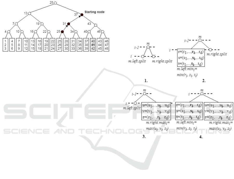
Let us suppose that the node 25 is the random
chosen node therefore the findStartingNode starts its
elaboration from it. Since,
and
the algorithm moves to the
node 31. Again, both conditions are false and the next
node is 37. The findStartingNode returns the node 37
because
. Please note that the
point 41 belongs to a bucket in the subtree of node 37.
Figure 1: The starting node returned by findStartingNode
with the query point and starting in the random
chosen node 25.
2.2.4 The Starting Node Property (SNP) for
K-D Trees
In order to affirm the SNP from k-d trees the
following definition needs:
Definition 1 (Stripe): Let
be a
query point and suppose that is an internal node.
Consider the following conditions:
1. If both and are internal node
in the same level, they have the same splitting
coordinate i = m.left.splitCoordinate=
m.rightCoordinate (figure 2.1):
(3)
(If swap them)
Here p
i
is the i-th coordinate of p.
2. If is a leaf and is internal i =
m.right.splitCoordinate (figure 2.2):
(4)
(If
swap them)
3. If is a internal and is leaf i =
m.left.splitCoordinate (figure 2.3):
(5)
(If
swap them)
4. If both and are leaves i =
m.splitCoordinates (figure 2.4):
(6)
(If
swap them)
Where
(
) is the maximum
(minimum) value of the i-th coordinate of the points
contained in the bucket of . If one of the condition
(3), (4), (5) and (6) holds the node is a stripe with
respect the i-th coordinate (i-stripe) for . In the
above definition the first three sub-condition
considers the cases in which at most one child of is
an internal node. In these cases the split coordinate of
that child is used. Instead, in the last case both
children are leaves and the split coordinate of itself
is used.
Figure 2: The four cases listed in the definition of the stripe
with respect the i-th coordinate (definition 1).
The SNP for k-d tree is the following:
SNP for k-d trees: Let = {
1
,…,
j
} the set
of the nodes visited at least once by the KN algorithm
on k-d tree and
the query point.
If node contains in its subtree a stripe for each
coordinate of .
Proof of SNP for k-d trees: For the sake of
simplicity, suppose , with higher number of
dimensions the proof is the same.
Let
be the query point. If the SNP
holds for a node then there must exist two node
and , such that they are respectively stripe for the x-
coordinate and y-coordinate. That is, minSplit
x
≤ p
x
≤
maxSplit
x
and minSplit
y
≤ p
y
≤ maxSplit
y
. Where
minSplit
i
(maxSplit
i
) is the value on the right (left)
side of one the inequalities (3), (4), (5) or (6).
Suppose, without loss of generality, that as an
ancestor of . Since the subtree of contains all
points having the x-coordinate in the range from
An Efficient Decentralized Multidimensional Data Index: A Proposal
235
minSplit
x
to maxSplit
x
and the subtree of contains
all points having the y-coordinate in the range from
minSplit
y
to maxSplit
y
then the subtree of contains
or the closest point to . If the KN does not visit
it returns an incorrect result then Since the
path from root to contains both and then also
. Let be a randomly chosen node, the
findStartingNode algorithm for k-d trees is the same
as before except that it use the procedure
holdSNP4KD instead of holdSNP. The procedure
holdSNP4KD is the following:
Procedure holdsSNP4KD(n)
i = getCoordinateIndex()
if isStripe(n, i)
stripes[i] = true
if allStripes()
return true
end if
end if
return false
End procedure
Where getCoordinateIndex() returns the i
coordinate as in the definition 1, stripes[] is an array
of boolean of size and allStripes() returns true only
if all elements in stripes[] are true. Of course, all
elements of stripe are initialized to false.
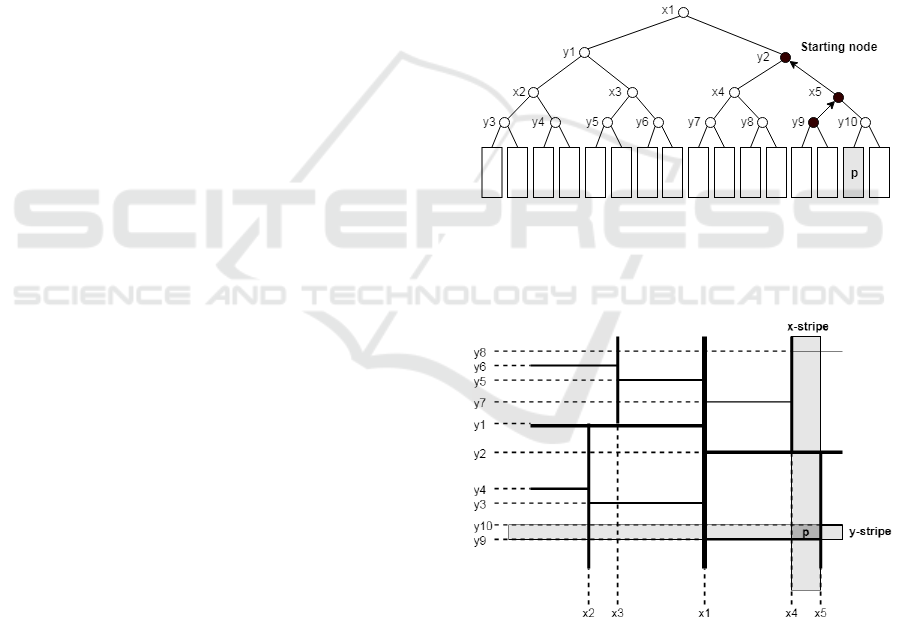
Example 2: Let’s consider the k-d tree in figure 3,
its planar representation in figure 4 and the query
point . Suppose that the chosen random node is .
Since,
then it is not
a starting node for and the algorithm moves to
It is
, but since the (3)
holds then is a y-stripe for (figure 4) and the
algoritm sets stripes[0] = true. Because AllStripes =
false the algorithm moves to and returns it as
starting node since is a y-stripe for and
AllStripes =true. The remaining part of the
description of the R-KN algorithm concerns the
condition to determine if a query has been completed
before reaching the root of the tree.
2.2.5 The Ending Node Property (ENP) for
Binary Trees
As already done for the Starting Node Property, first
the Ending Node Property for binary trees will be
introduced and it will be subsequently presented its
extension to k-d trees. Let
be a query
having two oolean attibutes: q.leftSideComplete and
q.rightSideComplete.
The R-KN algorithm follows the rule: suppose during
the ascending phase the R-KN comebacks to the node
from one of its children. If R-KN come from the left
(right) child of and the right (left) subtree of must
not be visited it set q.rightSideComplete = true
(q.leftSideComplete = true). If after the elaboration of
it holds that both q.leftSideComplete and
q.rightSideComplete are true then is an ending
node. In order to demonstrate that the R-KN can
terminate its elaboration in an ending node, we first
demonstrate that:
Theorem 4. Given a binary tree and a query
. If the KN ascends to the node from its left
child and the KN sets q.rightSideComplete = true
(q.leftSideComplete = true) in then in the remaining
steps of the KN no other right (left) subtree will be
processed. Intuitively, a point stored in a leaf in a right
subtree of an ancestor of is always more distant
from than a point in a leaf belonging to the subtree
of . Therefore, if the KN does not process the right
subtree of , it does not process any right subtree of
the ancestors of .
Figure 3: The resulting starting node returned by the
findStartingNode with the random chosen node y9 and
query point p.
Figure 4: In the planar representation of the k-d tree, the
gray bands represents the two stripes obtained with the
findStartingNode starting in the random node y9. Note that
the point p resides in the intersection of the stripes.
Proof of therorem 4: Let be the list of
temporary results and the farthest point in from
. Because the KN comes back from the left child of
it holds that:
DATA 2018 - 7th International Conference on Data Science, Technology and Applications
236
(7)
Furthermore, since q.rightSideComplete = true
then:
(8)
Please, note that p < v.split because if it is true
then using (7) it holds that
and then
and
this contradicts (8). Now, suppose , if
is the right child of then we must move to the
parent of because itself is the right subtree of
and it was already processed. If is the left child of
then by definition of binary tree.
Therefore, it holds that
it follows that the right subtree of will not be
visited. Finally, since it is possible to apply the same
reasoning for each node in the path from to the root
the conclusion is that no other right subtree will be
visited.
Theorem 5 (Correctness of the R-KN with ENP
for binary trees). Given a binary tree and a query ,
if the R-KN algorithm stops its elaboration in the first
ending node it finds then it returns the correct
results to query.
Proof of theorem 5: Since is an ending node
then the KN algorithm does not visit any other left
subtree nor right subtree along the path from to the
root of the tree during the ascending phase (Theorem
4).
As for the SNP property, it is difficult calculate
exactly how many time the R-KN using ENP will
process the root. The same approach of SNP in order
to estimate the behavior of the R-KN algorithm is
used and in about 98% of cases the R-KN terminates
in a node other than the root.
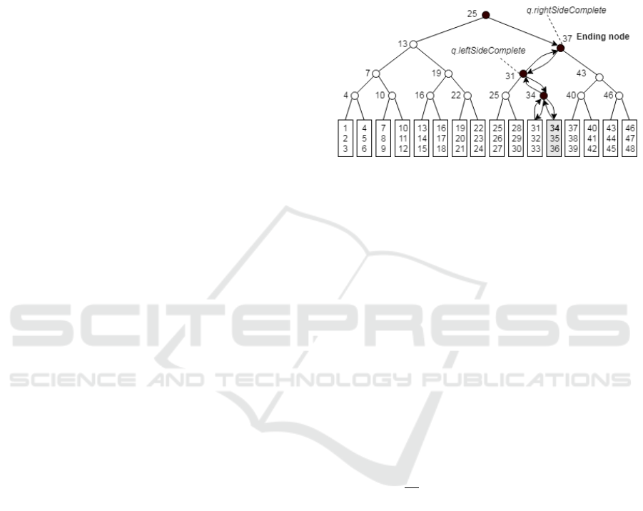
Example 3: Let’s consider the binary tree in figure
5 and the query
. Suppose the R-
KN starts in the root node. During the first
descending phase it visits nodes 37, 31 and 34. It
processes the leaf with bucket containing the query
point and it sets . The R-KN
ascends to node 34 and it checks the (1) since is
full. Since (1) holds, the algorithm process the other
sibling of 34 and it sets
(it throws
away the points 35 and 36 that are so far away from
). Now, R-KN comes back to node 34 and
since it processed both its children then the R-KN
ascends to node 31 and checks the condition (1).
Since
then the left subtree of
node 31 must not be visited. Here, the R-KN sets
. Intuitively, this
means that on the left side of the tree there are not
points belonging to the result of the query. Now, the
R-KN ascends to node 37 and again the condition (1)
is not true since
and the
algorithm sets . The
node 37 is an ending node and the algorithm
terminates. Please note that if R-KN starts in node 37,
instead of at the root, it returns also the correct result
since node 37 is a starting node for .
Figure 5: The ending node returned by R-KN with the query
point p = 34. In its ascending phase, R-KN sets
q.leftSideComplete = true in node 31 and finally it sets
q.rightSideComplete = true in node 37.
2.2.6 The Ending Node Property (ENP) for
K-D Trees
Let
be a query,
a -
dimensional point and q.leftSideComplete(i) and
q.rightSideComplete(i) two boolean array of size d.
The R-KN algorithm follows the rule: suppose during
the ascending phase the R-KN comes back to the node
from one of its children. If R-KN comes from the
left (right) child of and the right (left) subtree of
must not be visited it sets q.rightSideComplete(i) =
true (q.leftSideComplete(i) = true), where i =
v.splitCoordinate. If after the elaboration of it holds
that q.leftSideComplete(i) and q.rightSideComplete(i)
are true for all coordinates, then is an ending node.
Theorem 6 (Correctness of the R-KN with ENP
for k-dtrees). Given a k-d tree and a query
where
is a -dimensional point. If the
R-KN algorithm stops its elaboration in the first
ending node it finds, then it returns the correct
results to query.
Proof of theorem 6: The demonstration follows
from the observation that the Theorem 4 holds if we
consider a single dimension. Since is an ending
node, the Theorem 4 applies to all coordinates and
then no other subtree will be processed in the
remaining steps of the algorithm.
An Efficient Decentralized Multidimensional Data Index: A Proposal
237

3 RELATED WORKS
In the last decade multi-dimensional and high-
dimensional indexing in decentralized peer-to-peer
(P2P) networks, received extensive research
attention. In (Aly, 2011) there is proposal of a
distributed k-d tree based on MapReduce framework
(Dean, 2008). In such index structures queries are
processed similar to the centralized approach, i.e., the
query starts in root node and traverse the tree. These
methods exhibit logarithmic search cost, but face a
serious limitation. Peers that correspond to nodes
high in the tree can quickly become overloaded as
query processing must pass through them. In
centralized indexes this was a desirable property
because maintaining these nodes in main memory
allow the minimization of the number of I/O
operations. In distributed indexes it is a limiting factor
leading to bottlenecks. Moreover, this causes an
imbalance in fault tolerance: if a peer high in the tree
fails than the system requires a significant amount of
effort to recover. MIDAS (Tsatsanifos, 2013) is
similar to these works and in particular, MIDAS
implements a distributed k-d tree, where leaves
correspond to peers, and internal nodes dictate
message routing. MIDAS distinguishes the concepts
of physical and virtual peer. A physical peer is an
actual machine responsible for several peers due to
node departures or failures, or for load balancing and
fault tolerance purposes. A virtual peer in MIDAS
corresponds to a leaf of the k-d tree, and
stores/indexes all key-value tuples, whose keys reside
in the leaves rectangle and for any point in space,
there exists exactly one peer in MIDAS responsible
for it. Two algorithms for Nearest Neighbour Queries
are described: the first (expected
) has low
latency and involve a large number of peers; the
second (expected
) has higher latency but
involves far fewer peers. The proposed algorithms
process point and range queries over the
multidimensional indexed space in
hops in
expectance.
4 CONCLUSIONS
The main objective of this work is the proposal of
index with the following characteristics: 1) Must be
used on a large amount of data. The assumption is that
it is not possible or convenient to use a single
workstation to host all the data; 2) It is distributed
over a computer network and ensures the greatest
possible benefits in terms of efficiency (search, insert,
delete), i.e. the performance are close to the
traditional indexes that use a single workstation. The
basic ideas behind are a data structure, called
Decentralized Random Trees (DRT), based on k-d
tree and a novel k-nearest neighbour algorithm,
named random k-nearest neighbour algorithm. The
Decentralized Random Trees represent the main
contribution of this work. With a DTR distributed
over a network of peers a randomly chosen peer can
start the propagation of a query in the network
without involving the peer containing the root of the
tree in about 65% of cases. Furthermore, the first peer
that determines that the search is complete will return
the result. With high probability, more than 98% of
cases, that peer is not the peer containing the root. Of
course, due the distributed nature of the DRT, more
than one query can be running at the same time. The
number of initiated queries is potentially limitless
even if the number of peers limits the number of the
running queries.
REFERENCES
Abele, A., McCrae, J.P., Buitelaar, P., Jentzsch, A.,
Cyganiak, R., 2017. Linking Open Data cloud diagram
2017. http://lod-cloud.net/
Corley, C., Mihalcea, R., 2005. Measuring the semantic
similarity of texts. In Proceedings of the ACL workshop
on empirical modeling of semantic equivalence and
entailment (pp. 13-18). Association for Computational
Linguistics.
Faloutsos, C., Lin, k., 1995. FastMap: A fast algorithm for
indexing, data-mining and visualization of traditional
and multimedia datasets, volume 24. ACM.
Kruskal, J.B., Wish, M., 1978. Multidimensional scaling,
volume 11. Sage.
Gargiulo, F., Gigante, G., Ficco, M., 2015. A semantic
driven approach for requirements consistency
verification. International. Journal of High Performance
Computing and Networking, 8(3):201–211.
Basile, P., De Gemmis, M., Gentile, A.L., Lops, P.,
Semeraro, G., 2007. Uniba: Jigsaw algorithm for word
sense disambiguation. In Proceedings of the 4th
International Workshop on Semantic Evaluations,
pages 398–401. Association for Computational
Linguistics.
Samet, H., 2006. Foundations of multidimensional and
metric data structures. Morgan Kaufmann.
Aly, M., Munich, M., Perona, P., 2011. Distributed k-d
trees for retrieval from very large image collections. In
British Machine Vision Conference, Dundee, Scotland.
Dean, J., Ghemawat, S., 2008. MapReduce: simplified data
processing on large clusters. Communications of the
ACM, 51(1):107–113.
Tsatsanifos, G., Sacharidis, D., Sellis, T., 2013. Index-
based query processing on distributed
multidimensional data. GeoInformatica 17.3 pages:
489-519.
DATA 2018 - 7th International Conference on Data Science, Technology and Applications
238
