Option Pricing and Risk Hedging by Black-Scholes Model
and Cox-Ross-Rubinstein Model for Unilever PLC
Sen Chen
1,†
, Boyang Sun
2,*,†
and Jingzhe Lin
3,†
1
The College of Liberal Arts and Sciences, Arizona State University, 336E Orange St Tempe, AZ 85281, U.S.A.
2
Faculty of Science, University of Ottawa, 75 Laurier Ave E, Ottawa, ON K1N 6N5, Canada
3
Faculty of Environment & Faculty of Mathematics, University of Waterloo,
200 University Avenue West, Waterloo, ON, Canada
Keywords: Black Scholes Model, Cox-Ross-Rubinstein Model, Risk hedging, Python, Option pricing.
Abstract: Currently, option pricing and risk hedging are interesting topics in the financial field within the violate world.
This paper studies the performance of the different hedging strategies on options on stocks of Unilever PLC
within the Fast-Moving Consumer Goods Industry, which is helpful for both individual and institutional
investors to build their portfolios and choose a hedging strategy. In this study, implied volatility for each of
Unilever’s stocks is calibrated utilizing data on ten options on that stock. Then, with the Black Scholes Model
and Cox-Ross-Rubinstein model calculated, a hedging portfolio is composed, containing one unit of a specific
option and delta shares of the underlying stock for the company. Finally, the hedging performances of the
options on the company’s stocks are compared. The results in this paper benefit both individual and
institutional investors in choosing the best-fit hedging strategy depending on the nature of the underlying asset
to risk mitigation.
1 INTRODUCTION
To illustrate, a hedging strategy refers to a risk
management strategy that offsets losses in an
investment by taking the opposite position in a related
asset. As a matter of fact, hedging strategies are
widely used by individual investors as well as asset
management companies to mitigate risks and reduce
the extent of potential negative effects without
significantly reducing the rate of return. In addition,
as hedging strategies facilitate investors' investments
in more diverse assets, they help increase the liquidity
of their investments.
Within the numerous hedging strategies, using
options to hedge risks towards equity portfolios is
very critical and widely used, and its related topics
have long been studied, Galai analyzed the
components of the return from hedging options
against stocks (D. Galai, 1983). Also, Platen and
Schweizer provided a new explanation for the smile
and skewness effects in implied volatility from
hedging derivatives (E. Platen, 1998). Also, Bakshi,
*
Corresponding author
†
These authors contributed equally
Cao, and Chen compared the pricing and hedging of
short-term and long-term equity options (G. Bakshi,
2000), and Kumar studied the efficacy of option
Greeks and their significance in risk hedging
strategies (A. Kumar, 2018). Additionally, Howe and
Rustem presented a robust hedging algorithm to
hedge the risk of writing options (M.A. Howe, 1997).
Moreover, Soner, Shreve, and Cvitanic proved that
the least expensive method of dominating a European
call in a Black-Scholes model with proportional
transaction costs is the trivial strategy of buying one
share of the underlying stock and holding it to
maturity (H. M. Soner, 1995). Comparably, Gao, Li,
and Bai et al. also proposed an optimal risk hedging
strategy using put options with stock liquidity (R.
Gao, 2019). Becker, Cheridito, and Jentzen
introduced a deep learning method for pricing and
hedging American-style options as well (S. Becker,
2019).
In this study, the same delta-hedging strategy
utilizing the Black Scholes model and binomial tree
model is applied to a specific option on Unilever
Chen, S., Sun, B. and Lin, J.
Option Pricing and Risk Hedging by Black-Scholes Model and Cox-Ross-Rubinstein Model for Unilever PLC.
DOI: 10.5220/0012033500003620
In Proceedings of the 4th International Conference on Economic Management and Model Engineering (ICEMME 2022), pages 387-394
ISBN: 978-989-758-636-1
Copyright
c
 2023 by SCITEPRESS – Science and Technology Publications, Lda. Under CC license (CC BY-NC-ND 4.0)
387

Corporation’s stocks. And the hedging performance
on the company’s option is compared to give insights
into the difference in performances utilizing the same
hedging model across companies and sectors. The
results of this study show that the delta hedging
strategy utilizing the Black Scholes model and
binomial tree model performs well on selected
options.
2 DATA AND METHODS
2.1 Data
The data to be used are collected from Yahoo Finance
(https://ca.finance.yahoo.com). Data are used of five
call options and five put options on Unilever PLC
stocks collected from June 16th to July 18th, 2022,
which are used to calibrate implied volatility for the
stock of Unilever PLC. Unilever PLC, a mass
company with large volume and popularity in the
Fast-Moving Consumer Goods Industry, is supposed
to be representative of the FMCG industry. After
gathering data, a hedging strategy is constructed for
another option in this stock from June 27, 2022, to
July 8, 2022. The ten options used for calibration are
in-the-money, at-the-money, and out-of-the-money,
with similar prices to ensure that the sum of the
standard error is not so large that it is difficult to
calibrate implied volatility. The options information
collected to calibrate the implied volatility of
Unilever's stock is shown below in the table.
Table 1: 10 options chosen for calibration from uilever plc.
Call options
Unilever PLC
UL220819C000
40000
UL220819C000
42500
UL220819C000
45000
UL220819C000
47500
UL220819C000
50000
Puto
p
tions
Unilever PLC
UL220819P000
40000
UL220819P000
42500
UL220819P000
45000
UL220819P000
47500
UL220819P000
50000
The information on the option used for hedging is
shown in the table below.
Table 2: Option that is chosen for hedging for unilever plc..
Option
Unilever PLC UL220819C00037500
In addition to this, Unilever's share price from
June 17, 2022, to July 18, 2022, is shown below.
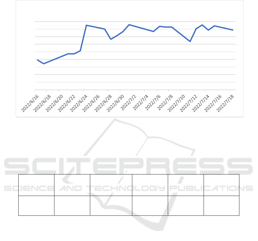
Table 3: Stock price of Unilever plc from June 16th,2022, to July 18th,2022.
Date (YYYY/MM/DD) The stoc
k
price of Unileve
r
PLC ($)
2022/6/16 43.96
2022/6/17 43.72
2022/6/21 44.37
2022/6/22 44.37
2022/6/23 44.57
2022/6/24 46.25
2022/6/27 46
2022/6/28 45.33
2022/6/29 45.56
2022/6/30 45.83
2022/7/1 46.29
2022/7/5 45.84
2022/7/6 46.18
2022/7/7 46.13
2022/7/8 46.13
2022/7/11 45.18
2022/7/12 46.02
2022/7/13 46.27
2022/7/14 45.93
2022/7/15 46.21
2022/7/18 45.94
ICEMME 2022 - The International Conference on Economic Management and Model Engineering
388

These data are plotted as a linear graph as shown
below.
Figure 1: Stock price trend of unilever plc.
As shown in the figure above, Unilever's share
price has a clear upward trend from June 14, 2022, to
June 24, 2022, rising from $43.96 per share to $46.25
per share, after which the share price remains
relatively stable, there was no obvious rise or fall, and
some volatility appeared during the period. The stock
price remained roughly at around $46 per share these
days.
Table 4: Descriptive statistics of the rate of return of stocks of unilever plc.
MEAN
STANDARD
DEVIATION
MEDIAN 1
ST
QUARTILE 3
RD
QUARTILE
UNILEVER PLC 43.72 0.8288782 45.93 45.18 46.13
As shown in the figure above, the average value of
this group of data is $43.72, while the median is
$45.93. The average value is smaller than the median
value, indicating that this group of data has an extreme
minimum value, and it also implies that Unilever’s
stock price does rose.
2.2 Methods
There are two steps to do with this study. The first step
is to bring the ten options used for calibration into the
Black-Scholes model and the Cox-Ross-Rubinstein
model to calibrate the implied volatility. The second
step is to substitute the calibrated implied volatility
into the formulas for calculating the delta value and
calculating the profit to calculate the profit of the
portfolio without hedging and the profit of the
portfolio with hedging, to test the effectiveness of the
hedging strategy that is constructed by the specific
option mentioned in the data part.
Above all, the Black-Scholes model reduces the
underlying asset and derivatives markets to a set of
rules expressed through mathematical formulas. This
model is widely cited around the world today and is
the basis for most market analyses. This model makes
pricing based on objective data. Objective data
include the time value of the option, the current price
of the asset on which the option is based; the strike
price on the maturity date of the option; and the
volatility of the asset price, which in turn can be
regarded as the probability that the option can be
executed. Despite many considerations, the model
does not require a complex computational process to
compute. However, the Black-Scholes model is not
perfect. The model is limited to calculating European
option prices. In some cases, the model cannot match
actual market conditions, unrealistic factors include
42
42,5
43
43,5
44
44,5
45
45,5
46
46,5
Unilever PLC
($)
Option Pricing and Risk Hedging by Black-Scholes Model and Cox-Ross-Rubinstein Model for Unilever PLC
389

the following: the model assumes that interest rates
are risk-free; volatility is known and constant; pricing
does not take into account transaction costs or taxes;
pricing does not take into account any dividends that
may be received by holders of the underlying asset.
Implied volatility reflects the level of uncertainty
or risk in the market and typically affects option
prices. Implied volatility is calculated by substituting
the traded option price into the price model and
inversely deriving the volatility value. First, a Black-
Scholes model is used to calibrate implied volatility.
The stock prices, expiration date, and strike prices of
all ten options used to calibrate implied volatility are
collected, and all stock prices from June 16 to July 18
are collected, and their standard deviation is
calculated to serve as the σ in the Black-Scholes
model with the formula below. σ represents the
implied volatility in the calibrated model but should
be assumed as a number to be substituted in the
calibration process, 𝑡 represents the time to maturity,
𝑆(𝑡) represents the stock price, 𝐾 represents the strike
price of each option, r represents the interest rate of
each option, here it is assumed to be zero as for the
time to maturity is quite short. Equation (1) and
equation (2) below calculate the prices of call options
and put options respectively, equation (3) and
equation (4) below represent the formula to calculate
𝑑1 and 𝑑2, which are the probability factors in the
Black-Scholes model, and 𝑁(𝑑1) and
𝑁
(
𝑑2
)
represent the normal distribution of d1 and d2
respectively (L.S. Lima, 2021; S. Ampun, 2021).
𝐶=𝑁
(
𝑑1
)
𝑆
(
𝑡
)
−𝑁
(
𝑑2
)
𝐾𝑒

(1)
𝑃=𝑁
(
−𝑑2
)
𝐾𝑒

−𝑆
(
𝑡
)
𝑁(−𝑑2)
(2)
𝑑1 =
𝐿𝑛
𝑆
(
𝑡
)
𝐾
+𝑟+
σ

2
t
𝜎
√
𝑡
(3)
𝑑2 =
ln
𝑆
(
𝑡
)
𝐾
+𝑟−
𝜎

2
𝑡
𝜎
√
𝑡
=𝑑1−𝜎
√
𝑡
(4)
The option prices calculated by the Black-Scholes
model will be compared with the actual market prices
of options, and the sum of standard error will be
calculated by equation (5), where 𝑃

(𝐵) represents
option prices that are calculated by the Black-Scholes
model, 𝑃

(
𝑀
)
represents market prices of options.
The implied volatility will be calibrated by
minimizing the sum of standard error.

(𝑃

(
𝐵
)
−𝑃

(
𝑀
)
)

𝑃

(
𝑀
)



(5)
The second, the Cox-Ross-Rubinstein model, also
named the binomial tree model, supposes that the
stock price fluctuates only in two directions, up and
down, and assumes that the range of up or down
fluctuations in the stock price remains unchanged
during the whole period. The model will divide the
entire period into several stages, simulate all possible
development paths of the underlying assets during the
whole duration based on the historical volatility of the
stock price, and calculate the option exercise profit
and usage for each node on each path. The option
price is calculated by the discount method. Compared
with the Black-Scholes model, the option pricing by
the Cox-Ross-Rubinstein model is more intuitive and
simpler to calculate, it can be applied to the pricing of
European options, American options, and some other
options. Moreover, the Cox-Ross-Rubinstein model
takes into account the interest rates and dividends
available to the underlying holders. The disadvantage
is that, when there are too many stages, that is, the step
size is too large, which will cause calculation
difficulties; when there are too few stages, that is, the
step size is too small, will reduce the accuracy, and the
gap between the market price and the actual price will
inevitably be large.
To be started, a Cox-Ross-Rubinstein model is
used to calibrate the implied volatility. Since the time
to maturity is relatively short, the 2-step binomial
option pricing model is used here, and the model has
still assumed the risk-free rate, which is denoted by
𝑟=0. In the Cox-Ross-Rubinstein model, ∆𝑡
represents the expiration time corresponding to the
options in each stage, u represents the multiplier when
the stock rises, d represents the multiplier when the
stock falls, and p represents the probability of the
stock rising. Equation (9) is used to calculate the stock
price in each layer, x represents the number of times
the stock increases, and 𝑆(0) is the original stock
price corresponding to the option. After that, compare
the calculated stock price with the strike price to
calculate the profit of option execution or non-
execution, calculate the probability of occurrence of
each income through the binomial formula, and add
the expected value of the profit to obtain the final
option price.
𝑢=𝑒

√
∆
(6)
𝑑=𝑒

√
∆
=
1
𝑢
(7)
𝑝=
𝑒
∆
−𝑑
𝑢−𝑑
(8)
𝑆(𝑥) = 𝑆(0)(𝑢

)(𝑑
()
)
(9)
ICEMME 2022 - The International Conference on Economic Management and Model Engineering
390

The option prices calculated by the Cox-Ross-
Rubinstein model are compared with the actual
market prices of options, and the sum of standard error
will be calculated by equation (5) above. Again,
𝑃

(𝐵) represents option prices that are calculated by
the Black-Scholes model, and 𝑃

(
𝑀
)
represents the
market prices of options. The implied volatility will
be calibrated by minimizing the sum of standard error.
Hedging strategies are formed against specific
options in Unilever stock after calibrating for implied
volatility. Then the collected Unilever PLC stock
price from June 27, 2022, to July 8, 2022, and the
implied volatility calibrated with each of the two
models are substituted into the following equations.
Equation (10) and equation (11) represent the
portfolio value of day 1 and each day after the first
day1, where 𝑁(𝑑1) in equation (11) uses the same 𝑑1
as the 𝑑1 in equation (3) and the algorithm is the same
as the Black-Scholes model, 𝑁(𝑑1) represents the
delta value of the option. The value of 𝑁(𝑑1)
changes with the changes in data each day, thus it
needs to be recalculated every day. Equation (12) and
equation (13) represent the loss without hedging and
the loss without hedging for each day.
Day1(June 27,2022)
𝑃𝑜𝑟𝑡𝑓𝑜𝑙𝑖𝑜 𝑣𝑎𝑙𝑢𝑒 X(1) = 𝐶(1,𝑆
(
1
)
)
(10)
Days after day1(June 28,2022-July 8,2022)
𝑝𝑜𝑟𝑡𝑓𝑜𝑙𝑖𝑜 𝑣𝑎𝑙𝑢𝑒 𝑋
(
𝑡
)
=𝑋
(
𝑡−1
)
+ 𝑁(𝑑1)(𝑆
(
𝑡
)
−𝑆
(
𝑡−1
)
)
(11)
𝐿𝑜𝑠𝑠 𝑤𝑖𝑡ℎ𝑜𝑢𝑡 ℎ𝑒𝑑𝑔𝑖𝑛𝑔(𝑡)
=𝑆
(
𝑡
)
−𝐾
−𝐶(1,𝑆
(
1
)
)
(12)
𝐿𝑜𝑠𝑠 𝑤𝑖𝑡ℎ ℎ𝑒𝑑𝑔𝑖𝑛𝑔(𝑡)
=𝑆
(
𝑡
)
−𝐾−𝑋(𝑡)
(13)
Compare the loss with hedging and the loss
without hedging calculated by the equations above, to
examine the difference between the two and the effect
of hedging.
3 RESULTS AND DISCUSSION
3.1 Results
First, substituting the implied volatility calculated by
the Black-Scholes model to calculate the profit before
and after hedging within the specific option of
Unilever PLC between June 27th, 2022, and July
11th, 2022. The comparison of trends for the two is
shown below.
Figure 2: Profit(loss) of unilever plc portfolio with calibration by black-scholes model.
-0,40000000
-0,20000000
0,00000000
0,20000000
0,40000000
0,60000000
0,80000000
1,00000000
2022.6.272022.6.282022.6.292022.6.30 2022.7.1 2022.7.5 2022.7.6 2022.7.7 2022.7.8 2022.7.11
Profit(Loss)
loss with hedging
loss without hedging
($)
Option Pricing and Risk Hedging by Black-Scholes Model and Cox-Ross-Rubinstein Model for Unilever PLC
391

The yield curve with hedging is shown close to a
straight line, parallel to the x-axis, which indicates
that the effect of hedging is relatively good, and the
volatility of returns is effectively reduced, which also
implies that the risk of options is reduced, and the risk
is close to zero, which avoids the loss of the option.
However, the disadvantages also emerged. As the risk
approaches zero, the option profit also decreases. The
profit with hedging was basically below 0.2, while the
high point of the income before hedging is around 0.8,
and the frequency was twice. In the statistics of time,
the profits with hedging are higher than the profits
without hedging in only four days, and the profits
without hedging of these four days are in a state of
loss. However, although there are four days of
negative option returns, it still does not affect the sum
of benefits brought by high returns without hedging is
higher than the sum of returns with hedging.
Figure 3: Profit(loss) of unilever plc portfolio with calibration by cos-ross-rubinstein model.
Option hedging strategies based on implied
volatility calibrated with a Cox-Ross Rubinstein
model also performed well. Its performance is roughly
equivalent to the option hedging strategy based on the
implied volatility calibrated by the Black-Scholes
model, and profit with hedging is basically a straight
line parallel to the x-axis, which proves that it
successfully hedged the fluctuation of the option price
and keeps the return value at a positive number, while
it also means that the risk is reduced, and the
possibility of high returns is also reduced at the same
time. As shown in the figure, although the hedging
returns continue to remain positive, the returns are
close to zero. From the comparison of the curve
amplitudes in the graph, the hedging strategies based
on Cox-Ross-Rubinstein model-calibrated implied
volatility seem to have lower returns than that of
hedging strategies based on Black-Scholes model-
calibrated implied volatility, which also means that
their returns are lower than hedges former strategy.
Table 5: The comparison of profits with hedging and profits without hedging of the specific option.
($)
2022/6/
27
2022/6/
28
2022/6/
29
2022/6/
30
2022/7/1 2022/7
/5
2022/7/6 2022/7/7 2022/7/8 2022/7
/9
sum
Profit
with
hedging
(Black-
Scholes
model)
0.0765
04
0.1003
22
0.0900
73
0.0796
25
0.064559 0.0758
90
0.06600
5
0.06716
8
0.06716
8
0.0867
79
0.7740
94
Profit
withou
t
0.0765
04
0.7465
04
0.5165
04
0.2465
04
(-)0.21349
6
0.2365
04
(-)0.103
496
(-)0.053
496
(-)0.053
496
0.8965
04
2.2950
39
-0,40000000
-0,20000000
0,00000000
0,20000000
0,40000000
0,60000000
0,80000000
1,00000000
2022.6.272022.6.282022.6.292022.6.30 2022.7.1 2022.7.5 2022.7.6 2022.7.7 2022.7.8 2022.7.11
Profit(Loss)
loss with hedging
loss without hedging
($)
ICEMME 2022 - The International Conference on Economic Management and Model Engineering
392

hedging
(Black-
Scholes
model)
Profit
with
hedging
(Cox-
Ross-
Rubinst
ein
model)
0.0149
80
0.0220
62
0.0186
12
0.0153
61
0.011089 0.0138
59
0.01124
11
0.01151
3
0.01151
3
0.0157
81
0.1460
10
Profit
without
hedging
(Cox-
Ross-
Rubinst
ein
model)
0.0149
80
0.6849
80
0.4549
80
0.1849
80
(-)0.27502
010
0.1749
80
(-)0.165
020
(-)0.115
020
(-)0.115
020
0.8349
80
1.6797
990
As can be seen from the figure, the total profit
brought by the hedging strategy using the implied
volatility calibrated by the Black-Scholes model from
June 2, 2022, to July 9, 2022, is $0.774094, the non-
hedging yield is $2.295039, which is higher than the
yield after hedging. The total income brought by the
hedging strategy using the implied volatility
calibrated by the Cox-Ross-Rubinstein model from
June 2, 2022, to July 9, 2022, is $0.146010, and the
non-hedging yield is $1.6797990, which is also
greater than the profits with hedging. In contrast, its
profit with hedging is lower than that of the hedging
strategy based on the implied volatility calibrated by
the Black-Scholes model.
3.2 Discussion
As for the results, hedging strategies constructed from
the implied volatility calibrated by the two models
performed well on the specific options of Unilever
PLC. This is reflected in the fact that both hedging
strategies keep the option return at a positive value,
and the return level is stable, a little higher than zero,
which means that the risk is well hedged. In order to
illustrate this point, first, volatility generally reflects
risk, and a relatively stable yield curve can better
reflect that risk has indeed been reduced. Second,
delta can also be understood in options calculation as
always, the probability of an option that can benefit or
lose. For instance, for an at-the-money option, the
delta value is generally around 50%. This is because
the stock price is equal to the strike price of the option
at a certain moment, and at the next moment, the stock
price is equal to the strike price of the option. It may
go up or down, and the probability of both is 50%. If
the stock price increases, then this at-the-money call
option becomes an in-the-money call option, and the
delta value will be higher than 50%. This option has a
greater than 50% probability of being exercised and
profiting. If the stock price decreases at the next
moment, this option will become an out-of-the-money
call option, and the delta value is less than 50%,
indicating that this option has a less than 50% chance
of being exercised and benefiting. The option selected
in this paper is an in-the-money call option with a
delta value higher than 50%, which implies that it has
a higher than 50% probability of being exercised and
benefiting on the expiration date. At the same time,
the object of this paper is Unilever PLC to represent
the FMCG industry. From July 2022 to August 2022,
the stock prices of most FMCG companies, including
Unilever PLC, have a slight upward trend. It can be
seen from the Unilever PLC stock price trend table in
the data section of this paper that when Unilever
PLC's share price rises, the delta value of the selected
in-the-money call option will inevitably rise, and the
possibility of profit is greater. When it is less than the
stock price at a certain moment, the possibility of
making a profit is also inevitable, which also shows
that the options profit without hedging increases and
is greater than the profits with hedging. The hedging
strategy made in this paper is to neutralize the delta
value and make it zero, which reduces the risk and
also inhibits the possibility of profiting by options.
Therefore, when the stock price is known to be rising
and the object of the hedging strategy is in the case of
in-the-money call options, it is inevitable that the
return after hedging is less than the return before
hedging, and the two hedging strategies with different
implied volatility make the level of the return curves
after hedging close to 0, indicating that they are well
achieved for the purpose of hedging delta.
In addition, it can be seen from the Results section
that the hedging strategies constructed by the implied
Option Pricing and Risk Hedging by Black-Scholes Model and Cox-Ross-Rubinstein Model for Unilever PLC
393

volatility calibrated by the two different models have
different returns. The implied volatility calibrated by
the Black-Scholes model is considered to have higher
accuracy because the Black -Scholes model itself has
the function of calibrating the implied volatility, and
the value of delta calculated in the hedging method
used in this paper is different from Black-Scholes are
closely related. The Cox-Ross-Rubinstein model may
not be very accurate in calculating the data in the
paper. This is because of its model characteristics. The
more stages this model has, the more accurate the
calibrated implied volatility will be. However, given
that the option expiration time is too short, this paper
adopts a 2- step volatility binary tree model, which
may cause certain errors in the calculation of implied,
hence the returns calculated by the two hedging
strategies with different implied volatility are slightly
different, however, it does not affect the good effect
of the hedging strategy constructed by the two.
4 CONCLUSION
Currently, option pricing and risk hedging are
interesting topics in the financial field. In this paper,
we combine the two issues for the Unilever PLC
stock. The empirical processes can be summarized as
follows. First, relevant data on the targeted asset is
carefully selected. Second, the Black Scholes Model
and Binomial Tree model are applied. Finally, the
hedging performance is compared for the two models,
and the results show that the related investors may
benefit from the hedging strategies when investing
Unilever PLC. However, deficiencies exist. For
example, option pricing models and hedging
strategies have numerous alternatives, in this paper,
limited methods are adopted, thus, applying other
models deserves further investigations.
REFERENCES
A. Kumar. A Study on Risk Hedging Strategy: Efficacy of
Option Greeks. Abhinav National Monthly Refereed
Journal of Research in Commerce & Management,
2018, 7(4), 77-85.
D. Galai. The components of the return from hedging
options against stocks. Journal of Business, 1983, 45-
54.
E. Platen, and M. Schweizer. On feedback effects from
hedging derivatives. Mathematical Finance, 1998, 8(1),
67-84.
G. Bakshi, C. Cao, and Z. Chen. Pricing and hedging long-
term options. Journal of econometrics, 2000, 94(1-2),
277-318.
H. M. Soner, S.E. Shreve, and J. Cvitanic. There is no
nontrivial hedging portfolio for option pricing with
transaction costs. The Annals of Applied Probability,
1995, 5(2), 327-355.
L.S. Lima and J.H.C. Melgaço. Dynamics of stocks prices
based in the Black & Scholes equation and nonlinear
stochastic differentials equations. Physica A: Statistical
Mechanics and its Applications, 2021, 581, 126220.
M.A. Howe, and B. Rustem. A robust hedging algorithm.
Journal of Economic Dynamics and Control, 1997,
21(6), 1065-1092.
R. Gao, Y. Li, Y. Bai, and S. Hong. Bayesian inference for
optimal risk hedging strategy using put options with
stock liquidity. IEEE Access, 2019, 7, 146046-146056.
S. Becker, P. Cheridito, and A. Jentzen. Pricing and
hedging American-style options with deep learning.
Journal of Risk and Financial Management, 2019,
13(7), 158.
S. Ampun, and P. Sawangtong. The approximate analytic
solution of the time-fractional Black-Scholes equation
with a European option based on the Katugampola
fractional derivative. Mathematics, 2021, 9(3), 214.
ICEMME 2022 - The International Conference on Economic Management and Model Engineering
394