Explainable Feature Learning with Variational Autoencoders for

Holographic Image Analysis

Stefan R

ohrl

1∗ a

, Lukas Bernhard

1∗ b

, Manuel Lengl

1 c

, Christian Klenk

2 d

, Dominik Heim

2 e

Martin Knopp

1,2 f

, Simon Schumann

1 g

, Oliver Hayden

2 h

and Klaus Diepold

2 i

Chair of Data Processing, Technical University of Munich, Germany

Heinz-Nixdorf Chair of Biomedical Electronics, Technical University of Munich, Germany

Keywords:

Quantitative Phase Imaging, Blood Cell Analysis, Machine Learning, Variational Autoencoder, Digital

Holographic Microscopy, Microﬂuidics, Flow Cytometry.

Abstract:

Digital holographic microscopy (DHM) has a high potential to be a new platform technology for medical

diagnostics on a cellular level. The resulting quantitative phase images of label-free cells, however, are widely

unfamiliar to the bio-medical community and lack in their degree of detail compared to conventionally stained

microscope images. Currently, this problem is addressed using machine learning with opaque end-to-end

models or inadequate handcrafted morphological features of the cells. In this work we present a modiﬁed

version of the variational Autoencoder (VAE) to provide a more transparent and interpretable access to the

quantitative phase representation of cells, their distribution and their classiﬁcation. We can show a satisfying

performance in the presented hematological use cases compared to classical VAEs or morphological features.

1 INTRODUCTION

Quantitative Phase Imaging (QPI) in combination

with microﬂuidics proves to be an extremely ﬂexible

method for the analysis of cellular samples (Nguyen

et al., 2022). The resulting optical tool allows re-

searchers to investigate kinetic and morphological

anomalies of cells free of labeling costs while pre-

serving a high amount of detail. The sample presen-

tation via a microﬂuidics cartridge leverages the ap-

proach to high throughput comparable to modern ﬂow

cytometry devices and therefore a profound statistical

validity. Hence, it is not surprising that the method

offers great potential in the research, diagnosis and

treatment of various diseases. Recent publications

https://orcid.org/0000-0001-6277-3816

https://orcid.org/0000-0002-5694-0902

https://orcid.org/0000-0001-8763-6201

https://orcid.org/0000-0002-4664-8107

https://orcid.org/0000-0001-8463-1544

https://orcid.org/0000-0002-1136-2950

https://orcid.org/0000-0002-7074-473X

https://orcid.org/0000-0002-2678-8663

https://orcid.org/0000-0003-0439-7511

These authors contributed equally to this work

This research was funded by BMBF ZN 01 | S17049.

in the medical ﬁelds of oncology (Lam et al., 2019;

Nguyen et al., 2017) and hematology (Paidi et al.,

2021; Ugele et al., 2018) are only a small subset of its

capabilities. Furthermore, advances in machine learn-

ing have also been applied to this discipline, enabling

automated processing, segmentation, and differentia-

tion for a wide variety of problems (Jo et al., 2019).

Besides their usage for improving the phase recon-

struction technique itself (Allier et al., 2022; Paine

and Fienup, 2018), big convolutional neural networks

(CNNs) surpassed many classical approaches for in-

stance segmentation and object classiﬁcation. These

black boxes show great performances for the retrieval

and analysis of blood as well as tissue cells (Midtvedt

et al., 2021; Kutscher et al., 2021).

Besides all their advantages, holography and a

microﬂuidics system for sample presentation entails

some new challenges. Performing a classical blood

smear, as the gold standard for hematological anal-

ysis, ensures a deﬁned orientation of the cells and a

precise alignment in the focal plane of a microscope

(Barcia, 2007). A microﬂuidics cartridge holds some

uncertainties here. In addition, there is the absence of

the usual color information and the lack to selectively

label individual cell components. Of course, it is still

possible to catch sight of a misaligned red blood cell,

but the differentiation of white blood cell (WBC) dif-

Röhrl, S., Bernhard, L., Lengl, M., Klenk, C., Heim, D., Knopp, M., Schumann, S., Hayden, O. and Diepold, K.

Explainable Feature Learning with Variational Autoencoders for Holographic Image Analysis.

DOI: 10.5220/0011632800003414

In Proceedings of the 16th International Joint Conference on Biomedical Engineering Systems and Technologies (BIOSTEC 2023) - Volume 2: BIOIMAGING, pages 69-77

ISBN: 978-989-758-631-6; ISSN: 2184-4305

 2023 by SCITEPRESS – Science and Technology Publications, Lda. Under CC license (CC BY-NC-ND 4.0)

ferentiation becomes impossible for the human eye.

Here, we want to enable human researches to re-

take control of the quality assurance in their cell se-

lection pipeline. Also, the classiﬁcation itself should

become more transparent as when using huge state

of the art CNNs. We present a fused approach of a

lightweight variational Autoencoder in combination

with a small classiﬁer, as this technique allows an as-

sessment of the underlying data and the decision mak-

ing process on a human like level of abstraction. Un-

intuitive low-level features are often incapable of de-

scribing the desired behavior of an analysis pipeline.

The Autoencoder approach provides an easy visual

interface and the ability to present an enormous data

set in a compact way. We demonstrate this behavior

in different experiments involving whole blood sam-

ples, puriﬁed white blood cells as well as defocused

and misaligned cells.

2 MICROSCOPY AND DATA SET

2.1 Digital Holographic Microscopy

A digital holographic microscope is capable of ob-

taining high-quality phase images of samples by using

the principle of interference between an object beam

and a reference beam. This makes it very interest-

ing for bio-medical applications (Jo et al., 2019) as

holography solves the problem of low contrast asso-

ciated with typical bright-ﬁeld microscopy caused by

the transparent nature of most biological cells. This

problem is usually overcome by staining or molecu-

lar labeling of cells, which requires time-consuming

preparation and analysis (Barcia, 2007; Sahoo, 2012;

Klenk et al., 2019). Phase images, on the other hand,

reveal much more detailed cell structures compared to

intensity images.

We use a customized differential holographic mi-

croscope by Ovizio Imaging Systems as shown in Fig-

ure 1. It enables label-free cell imaging of untreated

blood cells in suspension. Our approach is closely re-

lated to off-axis diffraction phase microscopy (Dubois

and Yourassowsky, 2015), but allows us to use a low-

coherence light source and does not rely on a refer-

ence beam. Precise focusing of cells is performed

with a 50×500 µm PMMA (polymethyl methacry-

late) microﬂuidics channel. We are using four sheath

ﬂows to center blood cells in the channel and avoid

contact with the channel walls. More detailed infor-

mation about the used holographic microscope can

be found in (Dubois and Yourassowsky, 2008) and

(Ugele et al., 2018).

Figure 1: The PMMA chip uses hydrodynamic focusing to

align the sample stream in the focal plane of the digital holo-

graphic microscope.

20 µm

(a) Raw Phase Image.

20 µm

(b) Background Subtraction.

20 µm

(d) Filtering.

Figure 2: Several pre-processing steps are required to obtain

clean image patches of individual cells.

2.2 Pre-Processing

The microscope setup provides quantitative phase im-

ages with a size of 512×384 pixels containing multi-

ple cells. We apply several pre-processing steps to

obtain isolated image patches, which contain the in-

dividual cells. Figure 2a shows an example of an un-

processed phase image of white blood cells in the mi-

croﬂuidics channel.

2.2.1 Background Subtraction

To remove background noise and artifacts of the

microﬂuidics channel, background subtraction is re-

quired. The background is estimated using the me-

dian of 1,000 images, which gives much better results

compared to using the mean. Due to the ﬁxed ori-

entation of the lens, camera, light, and microﬂuidics

channel, the background is assumed to be static over

the whole recording. As a result of background sub-

traction Figure 2b clearly shows a minimized expres-

sion of noise and artifacts compared to the raw image.

BIOIMAGING 2023 - 10th International Conference on Bioimaging

2.2.2 Segmentation

To ﬁnd the important regions of the image that con-

tain cells, we apply a binary thresholding to the phase

images. Here, a phase shift threshold of 0.3 rad

provides good results for ﬁltering out small debris.

From the resulting binary images, we extract the con-

tours of each region of interest using the OpenCV

findContours implementation of the algorithm pro-

posed by (Suzuki and Abe, 1985). As Figure 2c

shows, not only valid cells are identiﬁed by this rather

simple method of object detection.

2.2.3 Filtering

Debris and smaller cell fragments are likely to con-

tain enough optical mass to be sensed by the thres-

holding procedure. Therefore, a ﬁrst simple size ﬁl-

ter is applied, so only contours covering more than

30 pixels are stored with the corresponding 48×48

pixel image area around their center. An exemplary

result containing six valid cells can be seen in Fig-

ure 2d. Whereas this task could also be solved by the

proposed approach, this ﬁltering step restricts the va-

riety of events and simpliﬁes the convergence of the

used machine learning models, allowing us to employ

smaller neural networks.

2.3 Data Sets

All samples used in this work are provided by three

healthy donors

while keeping the measurement pro-

tocols as consistent as possible. Since our microscopy

approach illustrated in Section 2.1 works label-free

and therefore does not require any sample prepara-

tion, the whole blood (2.3.2) and defocused (2.3.3)

data set were measured within 15 minutes after blood

collection. To minimize spatial coincidences of cells

a 1:100 diluted blood sample is used for the robust

microﬂuidics ﬂow focusing. To distill single fractions

of the ﬁve common types of white blood cells as a

ground truth, we isolate the cells for the leukocyte

(2.3.1) data sets. Therefore, these samples have an

additional preparation time of maximum three hours.

The measurement itself only takes less than two min-

utes for every sample resulting in more than 10,000

uncorrelated frames each. These frames are pre-

processed as outlined in Section 2.2 yielding the de-

sired phase image patches of single cells.

All human samples were collected with informed con-

sent and procedures approved by application 620/21 S-KK

of the ethic committee of the Technical University of Mu-

nich.

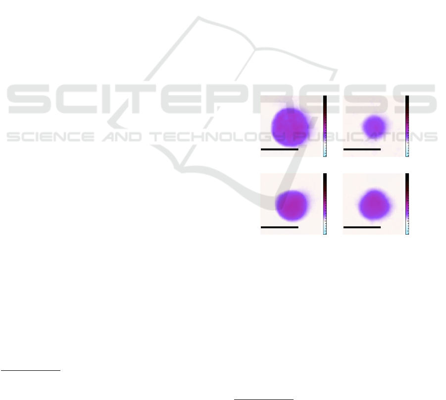
2.3.1 Leukocytes

Responsible for the immune defense, white blood

cells represent the most interesting group for the di-

agnosis of diseases and the general state of human

health. While making up only 1.5% of the total cell

count, these cells are in focus of every modern hema-

tology analysis device. These so-called leukocytes

can be divided in ﬁve major groups. For healthy indi-

viduals, Neutrophils (62%) make up the biggest pro-

portion, followed by Lymphocytes (30%), Monocytes

(5.3%), Eosinophils (2.3%) and Basophils (0.4%)

(Alberts, 2017; Young et al., 2013). We apply the

isolation protocol according to (Ugele, 2019; Klenk

et al., 2019): Starting from a whole blood sample

the leukocytes are separated from the red blood cells

using selective hypotonic water lysis as proposed by

(Vuorte et al., 2001). Remaining fragments are ﬁl-

tered out using an Erythrocyte Depletion Kit. Five

different Immunomagnetic Isolation Kits from Mil-

tenyi Biotec are then employed to obtain the individ-

ual fractions of WBCs. With this process we gathered

single cell images of 77,672 Lymphocytes, 58,760

Monocytes, 41,881 Eosinophils and 269,228 Neu-

trophils. Note that a 100% purity of those fractions

can not be ensured.

10 µm

−3

(a) Monocyte.

10 µm

−3

(b) Lymphocyte.

10 µm

−3

10 µm

−3

(d) Eosinophil.

Figure 3: The quantitative phase shift is color mapped in a

Giemsa stain (Barcia, 2007) fashion.

2.3.2 Whole Blood

Whole blood samples are of high value for many di-

agnostics as they do not require any sample prepara-

tion besides anticoagulants, which are already present

in a blood tube, and are therefore very close to in

vivo conditions. Omitting time consuming puriﬁca-

tion or staining steps facilitate insights to volatile ef-

fects in the sample. Mainly consisting of red blood

EDTA is used to prevent coagulation.

Explainable Feature Learning with Variational Autoencoders for Holographic Image Analysis

10 µm

−3

(a) RBC.

10 µm

−3

(b) Thrombocyte.

10 µm

−3

Figure 4: The whole blood samples contain besides white

blood cells mainly (a) red blood cells and (b) platelets. For

red blood cells the orientation (c) is crucial.

cells (erythrocytes), white blood cells (leukocytes)

and platelets (thrombocytes) are only a minority in

the human blood (Sender et al., 2016). Typical ex-

amples for red blood cells and platelets can be seen

in Figure 4. For comparability with the white blood

cells, we apply the same artiﬁcial Giemsa stain. The

viscoelastic focusing in the channel cannot guarantee

the alignment of the erythrocytes to the focal plane.

E.g. a tilted red blood cell as displayed in Figure 4c

cannot be used for malaria detection (Ugele, 2019).

The only preparation step for all whole blood sam-

ples is a dilution of 1:100 to facilitate the segmenta-

tion of individual cells. With the current laboratory

prototype and manual dilution step, results are ob-

tained within 15 min after blood draw. (Advanced

workﬂow integration could reduce the time-to-result

even further.) The whole blood data set contains a

total 126,480 images of single cells.

2.3.3 Defocused Cells

To simulate the behavior of unskilled measurement

personal, a technical defect or challenges of the opti-

cal setup (Cao et al., 2022), we created different cap-

tures from whole blood with a obviously misaligned

focus. We use the microscope stage to place the mi-

croﬂuidics channel and thereby the sample stream

at different offsets above as well as below the focal

plane of the objective. The misplacement ranges from

-10µm to +10µm with respect to the ideal focus. Fig-

ure 5 shows these clearly defocused images which are

again colored according to the previously introduced

scheme. As it may happen that individual cells get out

of focus even in a well calibrated setup, these images

serve as training set to detect this effect. These cells

are no longer usable for serious image analysis since

refocusing is impossible with our optical setup. With

this setting, we captured 7,269 examples of defocused

cells.

3 METHODOLOGY

Dimensionality reduction is an important area of un-

supervised learning. For high-dimensional data such

10 µm

−3

(a) -10 µm.

10 µm

−3

(b) −5 µm.

10 µm

−3

Figure 5: This data set contains cell images which where

captured with different focal offsets with respect to the ideal

focal plane.

as images, it is often necessary to reduce dimensional-

ity as a pre-processing step. This provides deeper in-

sight into the structure of the data and often improves

the performance of classiﬁcation or regression mod-

els. One of the most popular dimensionality reduction

techniques is principal component analysis (PCA),

which can provide deep insights into the most impor-

tant features of a data set (Jolliffe and Cadima, 2016).

The use of PCA implies an underlying linear sys-

tem, which cannot always be guaranteed. In contrast,

the Autoencoder approach used in this work repre-

sents an alternative, which, as a neural network, is not

bound to these assumptions (Schmidhuber, 2015). As

a deep-learning technique it utilizes non-linearly acti-

vated neurons which are organized in layers to encode

data samples into a compressed latent space (simi-

lar to principal components) and decode this compact

representation to recover the original data. The be-

havior and learned codes of an Autoencoder can be

affected by the number of codes (size of the latent

space) and hidden layers in use. It is important to note

that compared to PCA, which maximizes the variance

of the codes, the interpretation of the learned codes is

highly dependent on the trained data set.

3.1 Variational Autoencoder

Variational Autoencoders. (VAEs) introduce an ad-

ditional constraint to the latent space (Kingma and

Welling, 2013). The encoding should not only rep-

resent the original data as well as possible, but should

also follow a certain distribution (usually a Gaussian

distribution). This makes the latent space continu-

ous and allows sampling, which means we can gen-

erate artiﬁcial data by changing the value of the en-

codings. This generative behavior provides a deeper

insight into the learned feature representation, espe-

cially when sliding over an encoding (see Figure 7),

one can see the effect and its intensity of that feature

on the data at the output layer (Larsen et al., 2016).

The encoder is trained to encode the input data set X

into a distribution Q(z|X) represented by a mean vec-

tor µ

and a standard deviation vector σ

. This allows

sampling from that distribution to obtain an encod-

ing vector z which is fed into the decoder network to

BIOIMAGING 2023 - 10th International Conference on Bioimaging

create a reconstruction

X = P(X|z). Hereby, the en-

coder is forced to create codes following a prior dis-

tribution P(z) by including the Kullback-Leibler Di-

vergence D

of the learned distribution Q(z|X) and

the desired prior distribution P(z) in the loss function

of the VAE (Perez-Cruz, 2008). Hence, the loss

L (X,

X, z) = MSE(X,

X) + D

[Q(z|X)||P(z)] (1)

optimizes the reconstruction error under the con-

straint of a Gaussian distribution.

As we work directly on image data, the use of

convolutional layers instead of dense layers is ob-

vious, since these proved to be state of the art in all

sorts of image classiﬁcation and object detection tasks

over the last decade (Ciregan et al., 2012; Krizhevsky

et al., 2012). This leads to an improved representation

of spatial information in the VAE.

A well-known problem of VAEs are entangled

codes, which means that the codes are correlated and

a learned characteristic of the data is represented in

more than one encoding, leading to a reduced inter-

pretability of the latent space. Employing β-VAEs

addresses this problem (Burgess et al., 2018) by driv-

ing the network to disentangle its encodings using an

updated loss function

(X,

X, z) = MSE(X,

X) + β D

[Q(z|X)||P(z)].

(2)

Choosing β > 1 emphasizes the Kullback-Leibler Di-

vergence which forces z to be even more multivari-

ate Gaussian and consequently µ

→ 0 and σ

→ 1.

This reduces the correlation between the encodings z

leading to three important properties (Higgins et al.,

2017):

• z approximates a basis for the latent space Z

• The network is encouraged to use as few dimen-

sions of z as possible

• The latent space is smoothed out, improving the

generative behavior and allowing clearer interpre-

tations of the information stored in the encodings.

3.2 Classifying Variational Autoencoder

The aforementioned approaches do not incorporate

prior knowledge about the data samples and can learn

in an unsupervised way. Therefore, the trained en-

coder provides not necessarily clear and distinct clus-

ters in an interpretable manner. Conditional Varia-

tional Autoencoders allow to add another condition

c to the encoder Q(z|X, c) and decoder P(X|z, c) of

the VAE. This changes the latent space from a normal

distribution P(z) to a conditional distribution P(z|c),

yielding to some kind of class awareness of the en-

coder. Several publications showed the advantages of

this architecture as a generative model (Mishra et al.,

2018; Yan et al., 2016; Maaløe et al., 2016; Kingma

et al., 2014). Nevertheless, this turns into chicken-egg

problem for new samples, as a class label must be as-

signed to the unknown data point in order to be en-

coded correctly.

To overcome this problem we came up with a

new architecture to provide the VAE additional infor-

mation about labels during training while preserving

the encoding and generative nature of the VAE. The

classifying VAE (claVAE) is equipped with an ad-

ditional fully connected classiﬁer network

which is

connected to the µ

from the latent space as shown

in Figure 6. This provides the encoder and the latent

space with information about the ground truth labels

of the data, so that the encoder can optimally place the

data in the latent space by grouping samples of one

class together (path a) while maintaining a continu-

ous space from which we can sample (path b). The

decoder is responsible for reconstructing the original

image from the latent space (path c). Combining the

back-propagated errors along the three paths yields a

loss function

claVAE

(X,

X, z, y, ˆy) = L

(X,

X, z) + θL

BCE

(Y,

Y),

(3)

where θ controls the inﬂuence of the Binary Cross-

Entropy loss L

BCE

between the ground truth label Y

and the prediction

Figure 6: The claVAE architecture combines the classiﬁca-

tion error (a) the Kullback-Leibler Divergence (b) and the

reconstruction error (c).

3.3 Experimental Setup

For the training of the individual models, the de-

scribed data sets are divided into 60% training set (of

which 20% for validation) and 40% test set for the

evaluations shown later. Depending on the combi-

nation of data sets, the samples are balanced using

random undersampling according to their class label.

Inspired by https://www.datacamp.com/tutorial/

autoencoder-classiﬁer-python accessed Jan 16, 2020

Explainable Feature Learning with Variational Autoencoders for Holographic Image Analysis

The neural network architecture is kept constant be-

tween all models: The encoder (E) consists of four

convolutional layers with max pooling, two dropout

layers with a dropout rate of 0.25 and two dense layers

connected to z. The decoder (D) is implemented with

three dense layers to increase the dimensionality of

the bottleneck z and adapt it to ﬁve subsequent trans-

pose convolutional layers. The claVAE is addition-

ally equipped with a small dense classiﬁer network

a softmax layer as output. The parameters β = 0.1 and

θ = 1 to weight the components of the loss function

are chosen via a grid search and visual inspection of

the latent space. We could chose to encode more in-

formation by increasing the dimensions of the latent

space, striving for a better classiﬁcation accuracy. Ac-

cordingly, Figure 7 shows different kinds of character-

istics stored in each additional dimension of z ∈ R

Though we keep the latent space two-dimensional to

preserve its easy visualization and clarity.

−4 −2 0 2 4

Figure 7: A three-dimensional latent space can encode more

details of the input data. Here, one component of the latent

vector z

is varied, while the others z

and z

are kept at zero.

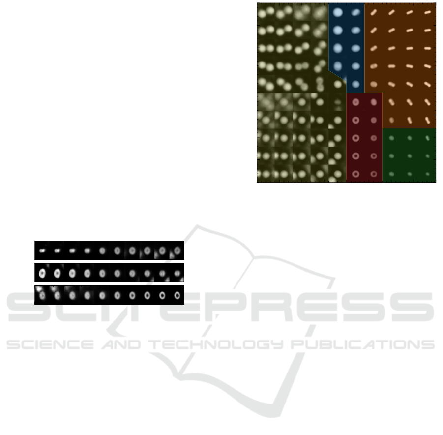
4 RESULTS

4.1 Overview

A typical workﬂow in a new project starts with getting

an overview. Therefore, we train the claVAE with all

data and labels introduced in Section 2.3. The result-

ing latent space in Figure 8 resembles a map for all

components of the presented blood samples, which

can be easily interpreted by the human observer. Re-

gion a) contains all defocused cells or cell aggregates.

These cells cannot easily be processed further in a

meaningful way and can be considered as outliers for

the scenarios presented in this work. Since they come

in a wide variety in shape and size, it is not surprising

that they occupy a large share in latent space. Reg-

ular shaped white blood cells and well-aligned red

blood cells can be found in the smaller areas b) and

d), respectively. The claVAE places red blood cells,

which might be unusable for further analysis as they

−4 −3 −2 −1 0 1 2 3 4

−4

−3

−2

−1

a) b) c)

Figure 8: The spatial representation of the cells in the latent

space of the claVAE can be partitioned in ﬁve groups: a)

defocused and doublets cells; b) WBCs; c) tilted RBCs; d)

RBCs; e) Platelets.

are tilted vertically, in sector c). It is visible how

the approach also tries to map the concept of orien-

tation. The last division e) contains only the smaller

cells like platelets or fragments. This arrangement is

quite stable over repeated iterations of training with

random initialization and randomly sub-sampled data

sets. The individual placement of the groups may vary

or the latent space might be rotated, but it can always

be used as an intuitive map to ﬁlter the cells of inter-

est for subsequent and more detailed analysis. We see

this way of pre-ﬁltering cells as a distinct advantage

over selection by morphological metrics, as it is more

similar to the established gating workﬂow. Further-

more, it allows a discussion of this processing step

on a higher level, which is more in line with human

nature to make decisions, especially in this interdisci-

plinary context.

4.2 Focus Detection

To make sure that no defocused cells get into the data

set, it is possible to sensitize claVAE to this appli-

cation case. We take well-focus WBCs b) and defo-

cused cells a) using the ﬁlters from before and pro-

vide the according labels from our training sets. Fig-

ure 9 shows the resulting distributions of the test set

in the latent space. We can see the well focused cells

mapped to the left whereas the defocused cells dom-

inate the right half plane. Aggregates of two or more

cells tend to be rather blurred, due to their size and the

limited optical depth of the microscope, and are there-

fore mapped more to the right. This can be seen by

BIOIMAGING 2023 - 10th International Conference on Bioimaging

−4 −3 −2 −1 0 1 2 3 4

−4

−3

−2

−1

Defocused

Focused

Figure 9: The density estimation of the test samples is eas-

ily separable due to the practical arrangement of the latent

space.

the smaller right-bound population originating from

the focused data set. The trained classiﬁer reaches

an accuracy around 96% when deciding if a cell is

well-focused or not. However, with this conveniently

arranged latent space, it would also be possible to use

simple logistic regression or a threshold as a decision

unit. Without the additional loss on the classiﬁcation

error, the training results from a β-VAE show a more

unstable behavior and consequently support the use of

the claVAE instead of a conventional variational Au-

toencoder.

4.3 Whole Blood Components

Considering only whole blood samples and puriﬁed

white blood cells for training, we aim to achieve more

detailed insights in the discrimination of RBCs and

WBCs. Both classes show a rather easy separability

in the latent space of this specialized claVAE. Drawn

in Figure 10 the RBCs populate the top part and the

WBCs are rather at the bottom.

Under the assumption that whole blood is prac-

tically RBCs, we neglected the other blood compo-

nents in our labeling. Looking at the apostate group of

RBCs, we hoped the claVAE would also ﬁnd WBCs

hiding under an incorrect ground truth label. Unfor-

tunately, the lower orange population consists of dou-

blet RBCs which where misplaced due to their bigger

appearance. The prolonged sample preparation time

and the special treatment of the puriﬁed WBCs might

have changed their appearance compared to the ones

in the untreated whole blood samples. However, the

classiﬁcation task in this space turns out to be rather

simple again, as the populations are basically linearly

separable. The employed classiﬁer can differentiate

both classes with an accuracy of around 97% based

−4 −3 −2 −1 0 1 2 3 4

−4

−3

−2

−1

WBC

RBC

Figure 10: WBCs and RBCs mostly populate different re-

gions of the latent space and are suitably distinguishable.

on their encoded representation.

4.4 Four-Part Differential

Getting more and more into the details of hematol-

ogy we now select only the available four single frac-

tions of WBCs as a training set. The rendering of

the latent space in the background of Figure 11 ﬁrst

suggests the distribution according to the size ratios

of the individual groups. As expected, the arrange-

ments of Neutrophils and Eosinophils overlap more

clearly, while the distributions for Lymphocytes and

Monocytes are better differentiated. Considering the

classiﬁcation performance already while training, the

four groups get pulled in different directions with re-

spect to the origin of the latent space. Using only the

β-VAE the mapping looks even worse. In general,

the overlapping regions lead to problems in classiﬁ-

−4 −3 −2 −1 0 1 2 3 4

−4

−3

−2

−1

Lym

Mon

Eos

Neu

Figure 11: The four leukocyte sub-populations are drawn

apart in the latent space of the claVAE but still overlap in

many areas.

Explainable Feature Learning with Variational Autoencoders for Holographic Image Analysis

cation. With this latent representation, the classiﬁer

network only reaches an accuracy of 74% performing

the four-part differential. Having a closer look at the

confusion matrix in Figure 12, it is evident that Neu-

trophils and Eosinophils get mixed up. Also Lympho-

cytes get partly confused with Eosinophils. Note that

a possible origin of this classiﬁcation error might be

the initial impurity of the ground truth labels them-

selves. The classiﬁcation performance could be im-

Lym Mon Eos Neu

Predicted label

Lym

Mon

Eos

Neu

True label

11695 603 2146 13

1390 12436 597 46

326 1118 9443 3487

1006 1829 2307 9249

2000

4000

6000

8000

10000

12000

Figure 12: The confusion matrix for the four-part differ-

ential reveals the respective classiﬁcation mistakes between

the cell types.

proved by allowing more dimensions for the latent

space, since two dimensions seem to be insufﬁcient to

preserve the precise details of the rater similar leuko-

cytes. Though, we choose not to do this as a high-

dimensional space would loose its intuitiveness and

would need a more complex interface for humans to

access it.

5 CONCLUSION

In summary, we can say that the developed approach

is well suited to obtain a compact overview of a large

data set. Researchers can use it to perform robust and

illustrative quality assurance as well as data cleaning,

as it is more intuitive and visual than nitpicking rules

of morphological features. In most of the demon-

strated use cases the claVAE generates clear and sep-

arable embeddings in its latent space, which can be

easily selected or classiﬁed. Its continuity and trans-

parency gives the method the potential to be more ro-

bust against outliers and unknown data compared with

large and opaque black-box approaches. In our inter-

disciplinary research, claVAE provides us with a basis

for “eye-level” exchange, even with people from out-

side the domain.

Yet, the method will never be totally accurate

since it would be necessary to sample the latent space

at an inﬁnitesimal level to prove its continuity. Even

if the latent space appears linearly separable and easy

to overlook, the employed encoder still uses a con-

volutional neural network, which cannot be fully ex-

plained and may hide some incontinuities. As we

chose the latent space two-dimensional, we fostered

its accessibility for human observers, but also lim-

ited the encoding power of the claVAE. This prevents

us from resolving the subtle differences in the white

blood cells needed for a classical ﬁve-part differential

with sufﬁcient accuracy.

Nevertheless, we plan to employ this non-linear

method for dimensionality reduction in a zoomable

user interface. Eventually, even novice users can get

an intuitive overview and perform gating in visual and

comprehensible manner. With further improvements

of DHM in the ﬁeld of label-free cell imaging, it is

to be expected that phase imaging ﬂow cytometry and

will be able to reach the high accuracy required for

automated hematology analysis.

ACKNOWLEDGMENTS

The authors would like to especially honor the contri-

butions of L. Bernhard for the software implementa-

tion and experiments as well as D. Heim and C. Klenk

for the sample preparation and measurements.

REFERENCES

Alberts, B. (2017). Molecular biology of the cell. WW

Norton & Company.

Allier, C., Herv

e, L., Paviolo, C., Mandula, O., Cioni,

O., Pierr

e, W., Andriani, F., Padmanabhan, K., and

Morales, S. (2022). CNN-Based Cell Analysis: From

Image to Quantitative Representation. Frontiers in

Physics, 9:848.

Barcia, J. J. (2007). The Giemsa stain: Its History and Ap-

plications. International Journal of Surgical Pathol-

ogy, 15(3):292–296.

Burgess, C. P., Higgins, I., Pal, A., Matthey, L., Watters,

N., Desjardins, G., and Lerchner, A. (2018). Un-

derstanding Disentangling in β-VAE. arXiv preprint

arXiv:1804.03599.

Cao, R., Kellman, M., Ren, D., Eckert, R., and Waller, L.

(2022). Self-calibrated 3D differential phase contrast

microscopy with optimized illumination. Biomedical

Optics Express, 13(3):1671–1684.

Ciregan, D., Meier, U., and Schmidhuber, J. (2012). Multi-

column deep neural networks for image classiﬁcation.

In 2012 IEEE Conference on Computer Vision and

Pattern Recognition, pages 3642–3649. IEEE.

Dubois, F. and Yourassowsky, C. (2008). Digital holo-

graphic microscope for 3D imaging and process using

it.

BIOIMAGING 2023 - 10th International Conference on Bioimaging

Dubois, F. and Yourassowsky, C. (2015). Off-axis interfer-

ometer.

Higgins, I., Matthey, L., Pal, A., Burgess, C., Glorot, X.,

Botvinick, M., Mohamed, S., and Lerchner, A. (2017).

beta-VAE: Learning Basic Visual Concepts with a

Constrained Variational Framework. In International

Conference on Learning Representations.

Jo, Y., Cho, H., Lee, S. Y., Choi, G., Kim, G., Min, H. S.,

and Park, Y. K. (2019). Quantitative Phase Imaging

and Artiﬁcial Intelligence: A Review. IEEE Journal

of Selected Topics in Quantum Electronics, 25(1):1–

14.

Jolliffe, I. T. and Cadima, J. (2016). Principal compo-

nent analysis: a review and recent developments.

Philosophical Transactions of the Royal Society A:

Mathematical, Physical and Engineering Sciences,

374(2065):20150202.

Kingma, D. P., Mohamed, S., Jimenez Rezende, D., and

Welling, M. (2014). Semi-supervised learning with

deep generative models. Advances in neural informa-

tion processing systems, 27.

Kingma, D. P. and Welling, M. (2013). Auto-encoding vari-

ational bayes. arXiv preprint arXiv:1312.6114.

Klenk, C., Heim, D., Ugele, M., and Hayden, O. (2019).

Impact of sample preparation on holographic imaging

of leukocytes. Optical Engineering, 59(10):102403.

Krizhevsky, A., Sutskever, I., and Hinton, G. E. (2012). Im-

agenet classiﬁcation with deep convolutional neural

networks. In Advances in neural information process-

ing systems, pages 1097–1105.

Kutscher, T., Eder, K., Marzi, A., Barroso, A., Schneken-

burger, J., and Kemper, B. (2021). Cell Detection

and Segmentation in Quantitative Digital Holographic

Phase Contrast Images Utilizing a Mask Region-based

Convolutional Neural Network. In OSA Optical Sen-

sors and Sensing Congress 2021 (AIS, FTS, HISE,

SENSORS, ES), page JTu5A.23. Optica Publishing

Group.

Lam, V. K., Nguyen, T., Phan, T., Chung, B.-M., Nehmetal-

lah, G., and Raub, C. B. (2019). Machine learning

with optical phase signatures for phenotypic proﬁling

of cell lines. Cytometry Part A, 95(7):757–768.

Larsen, A. B. L., Sønderby, S. K., Larochelle, H., and

Winther, O. (2016). Autoencoding beyond pixels us-

ing a learned similarity metric. In Proceedings of The

33rd International Conference on Machine Learning,

volume 48 of Proceedings of Machine Learning Re-

search, pages 1558–1566. PMLR.

Maaløe, L., Sønderby, C. K., Sønderby, S. K., and Winther,

O. (2016). Auxiliary deep generative models. In In-

ternational Conference on Machine Learning, pages

1445–1453. PMLR.

Midtvedt, B., Helgadottir, S., Argun, A., Pineda, J.,

Midtvedt, D., and Volpe, G. (2021). Quantitative dig-

ital microscopy with deep learning. Applied Physics

Reviews, 8(1):011310.

Mishra, A., Krishna Reddy, S., Mittal, A., and Murthy,

H. A. (2018). A generative model for zero shot learn-

ing using conditional variational autoencoders. In

Proceedings of the IEEE Conference on Computer Vi-

sion and Pattern Recognition Workshops, pages 2188–

2196.

Nguyen, T. H., Sridharan, S., Macias, V., Kajdacsy-Balla,

A., Melamed, J., Do, M. N., and Popescu, G. (2017).

Automatic Gleason grading of prostate cancer us-

ing quantitative phase imaging and machine learning.

Journal of Biomedical Optics, 22(3):036015.

Nguyen, T. L., Pradeep, S., Judson-Torres, R. L., Reed, J.,

Teitell, M. A., and Zangle, T. A. (2022). Quantita-

tive phase imaging: Recent advances and expanding

potential in biomedicine. American Chemical Society

Nano, 16(8):11516–11544.

Paidi, S. K., Raj, P., Bordett, R., Zhang, C., Karandikar,

S. H., Pandey, R., and Barman, I. (2021). Raman and

quantitative phase imaging allow morpho-molecular

recognition of malignancy and stages of B-cell acute

lymphoblastic leukemia. Biosensors and Bioelectron-

ics, 190:113403.

Paine, S. W. and Fienup, J. R. (2018). Machine learning

for improved image-based wavefront sensing. Optics

Letters, 43(6):1235–1238.

Perez-Cruz, F. (2008). Kullback-Leibler divergence esti-

mation of continuous distributions. In 2008 IEEE In-

ternational Symposium on Information Theory, pages

1666–1670.

Sahoo, H. (2012). Fluorescent labeling techniques in

biomolecules: A ﬂashback. Royal Society of Chem-

istry Advances, 2(18):7017–7029.

Schmidhuber, J. (2015). Deep learning in neural networks:

An overview. Neural Networks, 61:85–117.

Sender, R., Fuchs, S., and Milo, R. (2016). Revised esti-

mates for the number of human and bacteria cells in

the body. PLoS biology, 14(8):e1002533.

Suzuki, S. and Abe, K. (1985). Topological structural anal-

ysis of digitized binary images by border following.

Computer Vision, Graphics and Image Processing,

30(1):32–46.

Ugele, M. (2019). High-throughput hematology analy-

sis with digital holographic microscopy. PhD thesis,

Friedrich-Alexander-Universit

at Erlangen-N

urnberg

(FAU).

Ugele, M., Weniger, M., Stanzel, M., Bassler, M., Krause,

S. W., Friedrich, O., Hayden, O., and Richter, L.

(2018). Label-Free High-Throughput Leukemia De-

tection by Holographic Microscopy. Advanced Sci-

ence, 5(12).

Vuorte, J., Jansson, S.-E., and Repo, H. (2001). Evaluation

of red blood cell lysing solutions in the study of neu-

trophil oxidative burst by the DCFH assay. Cytometry,

43(4):290–296.

Yan, X., Yang, J., Sohn, K., and Lee, H. (2016). At-

tribute2image: Conditional image generation from vi-

sual attributes. In European Conference on Computer

Vision, pages 776–791. Springer.

Young, B., Woodford, P., and O’Dowd, G. (2013).

Wheater’s functional histology E-Book: a text and

colour atlas. Elsevier Health Sciences.

Explainable Feature Learning with Variational Autoencoders for Holographic Image Analysis