Model Fitting on Noisy Images from an Acoustoﬂuidic Micro-Cavity for

Particle Density Measurement

Lucas M. Massa

, Tiago F. Vieira

1 a

, Allan de M. Martins

2 b

Icaro B. Q. de Ara

ujo

1 c

Glauber T. Silva

and Harrisson D. A. Santos

Institute of Computing, Federal University of Alagoas, Lourival Melo Mota Av., Macei

o, Brazil

Department of Electrical Engineering, Federal University of Rio Grande do Norte, Natal, Brazil

Physics Institute, Federal University of Alagoas, Macei

o, Brazil

ﬁ

Keywords:

Particle Density Estimation, Genetic Algorithm, Gradient Descent, 2D Gaussian Fitting, Acoustoﬂuidics.

Abstract:

We use a 3D printed device to measure the density of a micro-particle with acoustoﬂuidics, which consists in

using sound waves to trap particles in free space. Initially, the particle is trapped in the microscope’s focal

plane (no blur). Then the transducers are shut off and the particle falls inside the ﬂuid, increasing its diameter

due to defocus caused by the distance to the lens. This increase in diameter along time provides its velocity,

which can, in turn, be used to compute its density. To manually annotate the diameter in the recorded images

is a tedious task and is prone to errors. That happens due to the high noise present in the images, specially

in the last frames where the defocus is high. Because of that, we use a 2D Gaussian model ﬁtting process to

estimate the particle diameter throughout different depth frames. To ﬁnd the diameters, we initially perform

the Gaussian parameters ﬁt with Genetic Algorithm in each frame of the recorded particle trajectory to avoid

local minima. Then we reﬁne the ﬁt with Gradient Descent using Tensorﬂow in order to compensate for

any randomness present in the ﬁt of the Genetic Algorithm. We validate the method by retrieving a known

particle’s density with acceptable performance.

1 INTRODUCTION

Separating particles of interest from complex mix-

tures is an important procedure done in many ﬁelds

such as biology (Fan et al., 2022) and medicine (Li

et al., 2015). Recently, acoustoﬂuidic, which consists

in using sound waves propagating through some ﬂuid

medium, has been used in areas like clinical diagnos-

tics (Wang et al., 2021) and therapeutics (Bose et al.,

2015) due to its capability of trapping particles having

speciﬁc physical characteristics. By observing iso-

lated particles or conglomerates (colloids), one can

conﬁrm the occurrence of speciﬁc reactions and de-

termine whether a given pathogen is present in a body

ﬂuid sample using a microscope, for instance.

Traditionally, several techniques have been used

to separate particles, such as those based on cen-

trifuges, which is time-consuming, can cause substan-

tial material loss and alter cell functions (Fan et al.,

2022). In contrast, with a carefully designed acous-

https://orcid.org/0000-0002-5202-2477

https://orcid.org/0000-0002-9486-4509

https://orcid.org/0000-0002-6769-4946

tic ﬁeld, one can separate target cells embedded in a

complex liquid, which has been validated as a viable,

contact-less, bio-compatible and label-free technol-

Figure 1: Captured images of a falling particle. The blur

gradually increases along the process. First row: original

images captured by a microscope. Middle row: Same im-

ages with enhanced contrast. Last row: particles ﬁtted by a

curve.

254

Massa, L., Vieira, T., Martins, A., Q. de Araújo, Í., Silva, G. and Santos, H.

Model Fitting on Noisy Images from an Acoustoﬂuidic Micro-Cavity for Particle Density Measurement.

DOI: 10.5220/0011670200003417

In Proceedings of the 18th International Joint Conference on Computer Vision, Imaging and Computer Graphics Theory and Applications (VISIGRAPP 2023) - Volume 4: VISAPP, pages

254-261

ISBN: 978-989-758-634-7; ISSN: 2184-4321

 2023 by SCITEPRESS – Science and Technology Publications, Lda. Under CC license (CC BY-NC-ND 4.0)

ogy. Additionally, by incorporating automation and

tackling limitations of conventional strategies, isolat-

ing sub-micron bio-particles can potentially acceler-

ate the development of Point-of-Care devices.

In this work, we use an acoustoﬂuidic 3D printed

device (ﬂuid chamber) to measure the density of

polystyrene beads. The device is initially ﬁlled with

a ﬂuid in which the analytes are embedded. Trans-

ducers are then excited to generate an acoustic ﬁeld

responsible for “trapping” the particle in a given po-

sition. A microscope is used to acquire images of the

cells as exempliﬁed in Fig. 1, where the “trapped” par-

ticle is represented by the ﬁrst image (top-left). After

the acoustic ﬁeld is disabled, the particle falls along

time, causing a strong blur as shown in the middle and

ﬁnal images in Fig. 1, since the particle is no longer

within the microscope focus plane. By observing the

fall velocity (depth per moment in time) and using a

calibration curve obtained in beforehand that relates

the particle’s diameter to depth, one can compute a

good estimate of the cell’s density (cf., Section 2).

Unfortunately, annotating cell’s diameters on dif-

ferent images is a manual process due to a very low

Signal-to-Noise Ratio (SNR) inherent to the blurring

process caused by the particle fall and short Depth-of-

Field of the microscope optical apparatus. Therefore,

one must manually annotate each image in both stages

of calibration and dynamic measurement. Manually

annotating images is a time-consuming and cumber-

some process due to many characteristics. It is prone

to human error and fatigue, rendering automation and

development of Point-of-Care devices unfeasible.

The bead’s diameter is related to the depth, which

can provide information regarding the velocity of the

fall (depth per time). It can be shown that the velocity

with which the particle falls into the medium, along

with other quantities can provide the particle’s den-

sity value (cf. Section 2). Therefore, we propose a

method capable of measuring the particle’s diameters

during its fall. Due to the amount of noise, we found

that ﬁtting a 2D Gaussian in a Gradient Descent fash-

ion can provide reasonable performance in the ﬁnal

densisty measurement.

Fitting a Gaussian onto a signal (image) is a

method that can be applied on different scenarios for

different purposes. For instance, Ananthanarasimhan

et al., used the technique to estimate the diame-

ter of discharges viewed by High Speed Cameras

(HSC) to characterize a rotating gliding arc (RGA)

reactor (Ananthanarasimhan et al., 2022). Kizel et

al. proposed a method for fully constrained spa-

tially adaptive spectral unmixing for the localiza-

tion of endmembers (Kizel et al., 2015). Lei et

al., used a 2D Gaussian ﬁtting procedure to lo-

cate motion-blurred, weak celestial objects in im-

ages (Lei et al., 2016) for the purpose of orbital de-

bris monitoring. Dai et al., used the method to es-

timate the Point Spread Functions of different opti-

cal apparatus and ultimately increase the resolution of

Single-Photon Emission Computerized Tomography

(SPECT) to sub-millimeter range (Dai et al., 2010).

Anniballe and Bonafoni proposed a Gaussian ﬁtting

procedure aimed at analyzing remotely sensed ther-

mal multi-resolution images to monitor variations in

urban occupancy throughout area and time (Anniballe

and Bonafoni, 2015). Bui et al., proposed the segmen-

tation of murine tumor from noisy ultrasound clinical

images using Gaussian distribution to model local in-

tensities (Bui et al., 2015).

In this context, we propose a Computer Vision

strategy capable of automatically measuring cell di-

ameter on noisy images using a simple, yet effective,

method based on 2D Gaussian ﬁtting using Genetic

Algorithm (GA) and a subsequent reﬁnement with

Gradient Descent (GD) method. Experiments showed

that the methodology provides a satisfactory perfor-

mance and can eventually contribute to the develop-

ment of fully automated devices.

2 EXPERIMENTAL

METHODOLOGY

The density of a particle embedded in a liquid affects

the rate in which it falls (in distance per time). The

relation between fall rate and density can be found by

analyzing the problem’s dynamics, which, for a parti-

cle embedded in a ﬂuidic medium, is ruled by a spe-

ciﬁc set of forces. As explained by (Zhao et al., 2014),

forces caused by particle-to-particle interaction, ther-

mal effects and Brownian motion can be disregarded

due to their low order of magnitude when compared

with other forces that act on the system. Thus, the

resulting force that pulls the particle down along the

vertical axis can be expressed as a combination of

gravitational, viscosity and buoyancy forces:

∑

−→

F =

−→

gravitational

−→

viscosity

−→

buoyancy

(1)

Considering that the vertical axis is pointed down-

ward and approximating the particle as a perfect

sphere, one can express the forces mentioned above

−→

gravitational



πgr

particle



k (2)

−→

buoyancy



−

πgr

f luid



k (3)

−→

viscosity

= (6πrµv)

k, (4)

Model Fitting on Noisy Images from an Acoustoﬂuidic Micro-Cavity for Particle Density Measurement

255

Microscope lens

Printed

Cylinder

Actuator

Resonant

Chamber

Printed

Cylinder

Resonant

Chamber

Confocal

plane

Levitated

particle

Standing

wave

Confocal

plane

Falling

particle

(a)

(b)

(c)

(d)

Cross-section cut

Actuator off

Actuator on

Figure 2: (a) Diagram of the used hardware. (b) Cross-section cut illustration of the device shown in (a). (c) When the actuator

is on, a standing wave is generated and the particle is trapped in the microscope confocal plane. (d) When the actuator is turned

off, the wave vanishes and the particle falls downwards presenting what we call a dynamic behaviour.

where ρ

particle

is the particle’s density, ρ

f luid

is the

ﬂuidic medium’s density, r is the sphere’s radius, µ

is the ﬂuid’s dynamic viscosity and v is the particle’s

velocity during fall.

Therefore, by applying Newton’s second law, con-

sidering v as particle’s velocity along z axis and solv-

ing the resulting differential equation for the intensi-

ties of the forces deﬁned above, the following expres-

sion is found (Zhao et al., 2014):

v(t) =

g(ρ

particle

− ρ

f luid

)

9µ

(1 −e

−

) (5)

Since τ = m/6πrηK is very small, the exponential

term from Equation (5) can be ignored. Manipulating

the resulting expression, one can ﬁnd the ﬁnal relation

between particle density and fall velocity:

particle

9µv

+ ρ

f luid

. (6)

I.e., one can compute the particle’s density (in kilo-

grams per cubic meters) if its fall velocity and its

radius are known. During the course of this work

we will analyze the dynamics of 10µm diameter

polystyrene beads, which have a well known density

of around 1050 kg·m

−3

2.1 Hardware

For the acoustoﬂuidic device, a cylindrical structure

was fabricated using a 3D printer (cf., Fig. 2a) (San-

tos et al., 2021). A small disk with a diameter of 4mm

and a height of 750µm was cast inside the cylindrical

structure and top sealed by a glass cover which also

acted as an acoustic reﬂector (cf., Fig. 2b). This disk

was used as an resonant chamber inside which parti-

cles were placed. A small inlet hole could be used

to ﬁll the chamber with ﬂuid solutions of particles.

This solutions could later be removed by an outlet

hole. To deliver our experiments we used a ﬂuidic

solution with density and dynamic viscosity values of

997 kg·m

−3

and 0.89×10

−3

Pa·s, respectively. At the

bottom of the acoustic chamber a circular piezoelec-

tric actuator, with a diameter of 25mm, was attached.

When the actuator is turned on, an acoustic standing

wave is produced inside the resonant chamber (cf.,

Fig. 2c). This creates an acoustic radiation force that

traps the particles in a standing wave node, which has

a height of approximately 95×10

−6

m from chamber’s

bottom. An optical microscope is placed above the

cylindrical structure such that confocal plane matches

the wave node where particles are levitated. Turning

off the actuator causes the acoustic forces to be ex-

tinguished (cf., Fig. 2d), so the particles fall within

the ﬂuidic medium. As the particles fall, they grad-

ually move away from microscope’s confocal plane,

becoming increasingly blurry in acquired images.

2.2 Pipeline for Single Particle

Conﬁguration

During the course of this work, the ﬂuidic solutions

introduced inside the acoustic chamber generally con-

VISAPP 2023 - 18th International Conference on Computer Vision Theory and Applications

256

tained around 100 particles. A particle-to-particle in-

teraction caused the appearence of grouped packs of

particles, which makes it difﬁcult to carry out the

experiments. To achieve a single-particle conﬁgura-

tion, a sequence of two steps was carefully followed.

Firstly, once a pack of particles started to emerge, the

actuator power was turned off. Lastly, about 10 sec-

onds later, the device was turned on again, causing

only a single particle to be trapped at the acoustic

wave pressure node. Through this pipeline the pro-

posed experiments could be successfully conducted.

2.3 Calibration

As it was already discussed, the density of a particle

can be measured by a model based on the fall pro-

cess inside a microﬂuidic cavity along with a confocal

optical inspection. As the particle falls, the relative

distance to the image confocal plane becomes larger.

This results in a blurring effect, which increases the

particle size in the image as it gets increasingly defo-

cused.

To analyze the dynamics of a particle with a spe-

ciﬁc diameter and unknown density, it is necessary to

use a calibration curve that relates the relative area

of a particle, which has the same diameter, with pre-

viously known heights between particle and the res-

onant cavity bottom during a fall process, as shown

in Fig. 4. Considering that we have n (in our exper-

iments we used 18 images for the callibration step)

acquired images from a particle during fall and its re-

spective heights and areas, relative area values can be

computed by the following equation:

relative

− A

(7)

where A

, A

and A

are, respectively, area values for

the ﬁrst, current and last captured images.

Therefore, the computed values for relative area

and height can be ﬁtted to a double exponential func-

tion, which is deﬁned as follows:

h = α

exp



−

relative



+ α

exp



−

relative



+ ω

(8)

where α

, α

, β

and ω

can assume arbitrary val-

ues, having no physical meaning. The resulting curve

can be later used to estimate height values for a new

particle by applying as input the relative area values

during a fall experiment. Lastly, we can derive the

obtained height values to estimate the falling velocity

for that particle and with Eq. (6), ﬁnd its density.

2.4 Curve Fitting

An important aspect of the particle area measurement

process is that it is done manually, being more sus-

ceptible to errors. This problem could be overcome

through the usage of a procedure to automatically

compute the particle area in the captured image. Aim-

ing to achieve such solution, during this step we inves-

tigated the feasibility of ﬁtting well known curves to

the particle area in an input image. The tests focused

mainly in the application of 2D Gaussian functions

for this task. The Gaussian is given by the following

expression:

z(x,y) = p exp

−



(x −µ

)

2σ

(y −µ

)

2σ



(9)

where:

• p: Gaussian amplitude.

• µ

: Position of the Gaussians center in the image

along the (horizontal) x-axis.

• µ

: Position of the Gaussians center in the image

along the (vertical) y-axis.

• σ: Standard deviation of the Gaussian (propor-

tional to the radius of the image)

The idea is to ﬁt the Gaussian model into the im-

age by minimizing the mean square error (MSE) be-

tween the Gaussian and each pixel in the image. This

technique is very powerful provided that the noise is

symmetric. Regardless of the amplitude of the noise

present in the image the model will have minimum

MSE only when the parameters of the Gaussian ﬁt as

best as possible with the object in the image.

Once ﬁtted, the Gaussian parameters can be used

to give us measures on the object like its position

(mean of the Gaussian) and size (standard deviation).

2.5 Genetic Algorithm

Deﬁning a Gaussian function that ﬁts to the particle

in an input image is not trivial. From Eq. (9), we can

consider p, µ

, µ

and σ

as curve parameters. Hence,

the task of ﬁnding values that best ﬁts an speciﬁc par-

ticle image becomes a non-convex optimization prob-

lem.

A common approach to perform optimization

tasks in such cases is the usage of Genetic Algorithms

(GA). This kind of algorithms are inspired by evolu-

tionist theory, where natural selection keeps alive only

the individuals that are more adapted to the environ-

ment and give them the opportunity to pass their genes

to future generations. As exposed by (Konak et al.,

Model Fitting on Noisy Images from an Acoustoﬂuidic Micro-Cavity for Particle Density Measurement

257

2006), in the GA formalism each individual is repre-

sented by a vector called chromosome. Chromosomes

vectors are formed by values called genes. Each chro-

mosome is considered to be a solution to the prob-

lem which is being optimized and are grouped in a set

called population. The chromosome vectors generally

are randomly initialized and through the combination

of their genes, in a iterative process, converge to an

optimized solution.

During this iterative process, two main operations

are conduced: crossover and mutation. Firstly, in the

crossover operation, two chromosomes combine their

genes to generate a new one. Lastly the mutation in-

troduces the chance of random changes to the genes,

which also happen in nature. At each iteration only

the most adapted individuals are used to perform the

crossover operation. This metric of how much an in-

dividual is adapted to the problem is called ﬁtness and

is calculated through a function that is deﬁned accord-

ing to the optimization problem necessities.

Hence, we tested a Genetic Algorithm approach

for the Gaussian function optimization. The popu-

lation was formed by chromosomes with the format

[p,σ

], which are parameters used to generate Gaus-

sian curves, as denoted by Eq. 9. During this step we

utilized 13 images of a single particle which were ac-

quired consecutively during the fall process. The par-

ticle initially appears clear and focused and gradually

blurs along the sequence of images. The following

preprocessing steps were done:

• Aligning the particle at the center of the image.

• Image resizing to a 32×32 shape.

• Subtraction of a mean background value.

Then, the resulting images were applied to the

genetic algorithm parameter optimization, which in-

tended to ﬁnd the best p and σ

values for a 2D Gaus-

sian function. As the particles were centralized by the

pre-processing steps, we ﬁxed the µ

and µ

parame-

ters to zero. The genetic algorithm was executed for

1000 generations, 100 individuals and a mutation rate

of 1%. The ﬁtness of each individual was measured

by the Mean Squared Error between the processed im-

age and the Gaussian curve created with the current

parameter values. This process was repeated for each

test image generating 13 sets of optimized p and σ

values.

2.6 Model Fitting Using Gradient

Descent Method

As the genetic algorithm is not deterministic, it may

not reach the global minimum of the error function.

Thus, a natural step is to apply a more controlled op-

timization method having as a starting point the best

parameters found for each image by the approach de-

scribed at Section 2.5. For this task we tested the

application of a Stocastic Gradient Descent (Bottou,

2012) optimizer for p and σ

parameters.

Considering that we have a particle image y and

we want to approximate it by a Gaussian curve

z(p,σ

), our goal is to ﬁnd p and σ

values that

minimize a chosen loss function L(z(p,σ

),y), which

evaluates how far the generated curve is from the de-

sired one. Differential calculus deﬁnes the gradient of

a function as a vector that indicates the direction to

move from the current input parameters point so that

one can get the greatest increase rate. Thus, one can

minimize the function value by moving to the oppo-

site direction, which is called gradient descent.

Therefore, assuming w = [p,σ

] as an input vec-

tor, we can minimize the loss by updating it’s values

in a iterative process by using the following expres-

sion

i+1

= w

− α∇

L(z(w),y) (10)

where α is called learning rate and is responsible for

determining the update step size at each iteration.

Taking into account that the genetic algorithm

achieved results close to a global minimum, the curve

gradient at this point will have very small values. To

tackle this scenario, we used a higher learning rate

value of 2.0. We also executed the process for 1000

epochs for each set of test images and initial parame-

ters and applied a Mean Squared Error loss function,

which, for two input images, can be deﬁned as fol-

lows:

MSE =

W H

W −1

∑

x=0

H−1

∑

y=0

[ f (x,y) − g(x,y)]

(11)

where W and H are, respectively, images’ width and

height values.

3 RESULTS AND DISCUSSION

3.1 Height and Relative Area Curve

By applying the proposed methodology, we were able

to obtain a calibration curve for the experiment. With

the usage of ground-truth images, where particle’s

contour was previously known, we extracted parti-

cle’s radius from a pixel-micron relation. Then, we

calculated area values by considering the particle as

a perfect circle and, along with it’s respective height

values, we could generate a calibration curve that re-

lated particle height with relative area, as discussed in

VISAPP 2023 - 18th International Conference on Computer Vision Theory and Applications

258

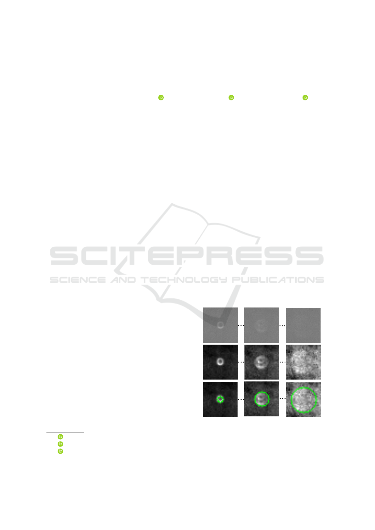
Figure 3: Image grid showing the results for diameter estimation. First row: Original images (last 8 slices from left to right

– ie. heights). Second row: Processed images. Third row: Contours obtained with the Genetic Algorithm. Bottom row:

Contours found using the Gradient Descent approach.

section 2.3. Numerically ﬁtting the points to the pro-

posed double exponential function (Eq. (8)), we could

achieve the curve shown in Fig. 4.

3.2 Genetic Algorithm and Gradient

Descent

After the application of the pipeline proposed in Sec-

tions 2.5 and 2.6, we could achieve good results for all

test images. Figure 3 presents an image grid contain-

ing results for eight of the thirteen tested images. De-

spite being stochastic, the genetic algorithm was able

to ﬁnd good parameters for the 2D Gaussian func-

tions. As shown in the second row of Fig. 3, the con-

tours of resulting Gaussian curves seem to ﬁt, if not

perfectly match, the particle contour. The results are

even more interesting for the last images of the se-

quence, where we ﬁnd a high amount of noise and a

Figure 4: Curve obtained by ﬁtting an exponential function

to height and relative area values during the calibration pro-

cess.

clear contour for the particle is not visually identiﬁ-

able. Still, the algorithm was able to ﬁnd plausible

parameters for the Gaussian curves as we can see in

Fig. 4.

The application of the Stochastic Gradient De-

scent optimizer did not change the results in general.

Despite giving a lower loss value, the resulting Gaus-

sian curve was practically the same. The only excep-

tions were the results for three of the thirteen test im-

ages, which are shown in fourth, seventh and eighth

columns of Fig. 3. The optimization produced a visi-

ble result, since curve contours changed slightly with

respect to the ones found by the genetic algorithm.

However, for all other images, the plotted Gaussian

contour was exactly the same, which ratiﬁes the good

result found by the genetic approach. In Fig. 5 we

can see resulting loss curves for the parameter tuning

process.

3.3 Density Measurement

Lastly, we used the obtained Gaussian curves to com-

pute particles’ areas in each image and generate rel-

ative area values by applying Eq. (7). Such values

could then be used as input for the calibration curve

discussed in Sections 2.3 and 3.1 to estimate particle’s

height at each image, which are shown in Figure 6.

Then, we numerically derived the height curve

and applied the mean value as particle’s velocity in

Eq. (6) to compute the particle’s density. For this

computation we also used a gravitational accelera-

tion of g = 9.82 m·s

−2

along with previously dis-

cussed values of ρ

f luid

= 997 kg·m

−3

and µ = 0.89 ×

Model Fitting on Noisy Images from an Acoustoﬂuidic Micro-Cavity for Particle Density Measurement

259

Figure 5: Example loss curves during the parameter opti-

mization process. Plots show, respectively, results for ge-

netic algorithm and gradient descent steps.

−1

Pa·s. This procedure resulted in a density value

of 1059 kg·m

−3

, which is close to the real density

value of 1050 kg·m

−3

, corresponding to an error of

0.8%.

Such result ratiﬁes our approach as a valid mean

to estimate the area of a particle and its density by ap-

plying the previously described equations. It is worth

mentioning that even in extreme cases, where the par-

ticle was not easily identiﬁable and the image con-

tained a lot of noise, the proposed method was capa-

ble of giving good estimates for Gaussian curve ap-

proximation for the particle, consequently allowing

the computation of it’s density.

4 CONCLUSIONS

We presented a methodology to obtain a sub-micron

particle’s density using acoustoﬂuidics. This ap-

proach is traditionally performed manually, which

renders the development of point-of-care devices un-

feasible.

Aiming at automating the process, we proposed

the use of 2D Gaussian ﬁtting to retrieve particle’s di-

ameters throughout different positions during fall as

an alternative to analyze its velocity and compute its

Figure 6: Estimated height for each image by applying com-

puted Gaussian areas as input to the calibration curve.

density. After a calibration procedure, the fall dynam-

ics was analyzed and the diameters were used as in-

puts to the calibration function in order to obtain the

corresponding depths along time. This fall velocity

is used alongside different parameters in a given for-

mulation to compute the density. Given a reference

known value of 1050 kg·m

−3

the method provided a

value of 1059 kg·m

−3

, satisfactorily close to the cali-

bration density. As future work, we intend to analyze

the usage of blur score metrics related to Gradient,

Laplacian, Fourier Transform and wavelets as an ap-

proach to the discussed particle ﬁtting problem.

ACKNOWLEDGEMENTS

This work was partially funded by SOFTEX

REFERENCES

Ananthanarasimhan, J., Raghuram, A., and Rao, L. (2022).

Arc diameter estimation of a rotating gliding arc using

a simple highspeed camera and gaussian ﬁt function.

IEEE Transactions on Plasma Science, 50(6):1401–

1406.

Anniballe, R. and Bonafoni, S. (2015). A stable gaussian

ﬁtting procedure for the parameterization of remote

sensed thermal images. Algorithms, 8(2):82–91.

Bose, N., Zhang, X., Maiti, T. K., and Chakraborty, S.

(2015). The role of acoustoﬂuidics in targeted drug

delivery. Biomicroﬂuidics, 9:052609.

Bottou, L. (2012). Stochastic gradient descent tricks. In

Neural networks: Tricks of the trade, pages 421–436.

Springer.

Bui, T. M., Coron, A., Mamou, J., Saegusa-Beecroft, E.,

Machi, J., Dizeux, A., Bridal, S. L., and Feleppa, E. J.

(2015). Level-set segmentation of 2d and 3d ultra-

sound data using local gamma distribution ﬁtting en-

https://softex.br/

VISAPP 2023 - 18th International Conference on Computer Vision Theory and Applications

260

ergy. In 2015 IEEE 12th International Symposium on

Biomedical Imaging (ISBI), pages 1110–1113.

Dai, T., Ma, T., Liu, H., Cui, J., Liu, Y., Wei, Q., Wu,

J., Wang, S., and Jin, Y. (2010). Low-cost high-

resolution animal spect imaging on a clinical spect

scanner. In 2010 3rd International Conference on

Biomedical Engineering and Informatics, volume 1,

pages 341–344.

Fan, Y., Wang, X., Ren, J., Lin, F., and Wu, J. (2022). Re-

cent advances in acoustoﬂuidic separation technology

in biology. Microsystems & Nanoengineering, 8:94.

Kizel, F., Shoshany, M., and Netanyahu, N. S. (2015). Spa-

tially adaptive hyperspectral unmixing based on sums

of 2d gaussians for modelling endmember fraction

surfaces. In 2015 IEEE International Geoscience and

Remote Sensing Symposium (IGARSS), pages 4440–

4443.

Konak, A., Coit, D. W., and Smith, A. E. (2006). Multi-

objective optimization using genetic algorithms: A

tutorial. Reliability engineering & system safety,

91(9):992–1007.

Lei, Z., Chen, X., and Lei, T. (2016). Sub-pixel location of

motion blurred weak celestial objects in optical sen-

sor image based on elliptical 2d gaussian surface ﬁt-

ting. In 2016 International Conference on Industrial

Informatics - Computing Technology, Intelligent Tech-

nology, Industrial Information Integration (ICIICII),

pages 100–104.

Li, P., Mao, Z., Peng, Z., Zhou, L., Chen, Y., Huang, P.-H.,

Truica, C. I., Drabick, J. J., El-Deiry, W. S., Dao, M.,

Suresh, S., and Huang, T. J. (2015). Acoustic sepa-

ration of circulating tumor cells. Proceedings of the

National Academy of Sciences, 112:4970–4975.

Santos, H. D. A., Silva, G. C., Vieira, T. F., Silva, A. E.,

de Ara

ujo, . B. Q., Jacinto, C., Rocha, U., Alexandre-

Moreira, M. S., and Silva, G. T. (2021). Measuring

cell density in a acoustoﬂuidic microcavity. In 2021

IEEE UFFC Latin America Ultrasonics Symposium

(LAUS), pages 1–4.

Wang, Z., Wang, H., Becker, R., Rufo, J., Yang, S., Mace,

B. E., Wu, M., Zou, J., Laskowitz, D. T., and Huang,

T. J. (2021). Acoustoﬂuidic separation enables early

diagnosis of traumatic brain injury based on circu-

lating exosomes. Microsystems & Nanoengineering,

7:20.

Zhao, Y., Lai, H. S. S., Zhang, G., Lee, G.-B., and Li, W. J.

(2014). Rapid determination of cell mass and density

using digitally controlled electric ﬁeld in a microﬂu-

idic chip. Lab Chip, 14:4426–4434.

Model Fitting on Noisy Images from an Acoustoﬂuidic Micro-Cavity for Particle Density Measurement

261