A Correlation Network Model for Analyzing Mobility Data in Depression

Related Studies

Rama Krishna Thelagathoti

and Hesham H. Ali

College of Information Science and Technology, University of Nebraska Omaha, Omaha, NE 68182, U.S.A.

Keywords:

Graph Models, Correlation Networks, Depression Studies, Mobility Data, Objective Diagnosis, Severity

Assessment.

Abstract:

Depression is a serious behavioural disorder that can affect the quality of life. Timely diagnosis and accurate

estimation of severity are critical in supporting depression studies and starting early interventional treatment.

In this study, we introduce two major contributions. First, we propose a novel computational model that

can utilize non-invasive mobility data to recognize individuals suffering from depression disorders. Second,

we introduce a new objective index, the Depression Severity Score Index (DSS), which can approximate the

seriousness or the degree of severity of depression. The proposed approach is a data-driven model that is

built on the mobility data collected from 55 subjects using wearable sensors. In the ﬁrst step in our proposed

approach, a graph model that represents the underlying correlation network is constructed by measuring the

pair-wise correlation values between each pair of individuals. Then, we obtain the depression severity index

of each subject by utilizing graph properties of the constructed network such as Intra and inter-cluster edges.

Our obtained results show that the obtained correlation network model has the potential to identify participants

diagnosed with depression from the control group. Moreover, the proposed Depression Severity Score (DSS)

has a higher likelihood than the clinical depression score in correctly measuring the depression severity level.

1 INTRODUCTION

In recent years, the prevalence of behavioral disorders

such as depression is in increasing trend. Especially,

During the COVID-19 pandemic, depression and anx-

iety disorders are more prevalent than usual in the

general population (Mazza et al., 2020). depression

would be the second most disability that most peo-

ple will suffer around the world (Mathers and Lon-

car, 2006). In addition to this, the cost of healthcare

would signiﬁcantly rise. Furthermore, recent studies

show that one out of every ﬁve young children is suf-

fering from at least one of the mental health issues

including depression, schizophrenia, and ADHD (Li

et al., 2021). However, only 25% of them are being

diagnosed and treated and the rest of them are undiag-

nosed. Besides, many children are not aware that they

are being affected by mental disorders. According to

National Institute of Mental Health (NIMH) statis-

tics, approximately 21 million people have at least

one major depressive disorder (unipolar or bipolar

https://orcid.org/0000-0002-4986-5027

https://orcid.org/0000-0002-8016-6144

depression) (The National Institute of Mental Health

(NIMH), 2021). Astonishingly, this number is almost

8% of the total US adult population.

Depression is characterized by a gloomy mood,

lack of interest in general everyday activities, low

self-esteem, and withdrawal from social gatherings

(Thelagathoti and Ali, 2022b) (Thelagathoti and Ali,

2022a). The prevalence of depression for a long time

may result in negative outcomes such as poor perfor-

mance in academics or work location, reduced mo-

bility, self-harm, and unemployment (Li et al., 2021).

Especially, suicidal thoughts and self-hurting would

dramatically increase. Therefore, it is crucial to iden-

tify the condition and facilitate the treatment as early

as possible. Without estimating the severity of the

depression, it is not viable to provide comprehensive

treatment. Assessment of the seriousness of the dis-

order is as critical as the detection of the disorder.

Nevertheless, most of the existing clinical procedures

are symptom rating scales such as the MADRS score

(Montgomery and

Asberg, 1979) and the Depression

Rating Scale (Williams, 1988). In these approaches,

severity is estimated by assigning a score or rating for

each of the symptoms that are expressed by the indi-

416

Thelagathoti, R. and Ali, H.

A Correlation Network Model for Analyzing Mobility Data in Depression Related Studies.

DOI: 10.5220/0011675400003414

In Proceedings of the 16th International Joint Conference on Biomedical Engineering Systems and Technologies (BIOSTEC 2023) - Volume 5: HEALTHINF, pages 416-423

ISBN: 978-989-758-631-6; ISSN: 2184-4305

 2023 by SCITEPRESS – Science and Technology Publications, Lda. Under CC license (CC BY-NC-ND 4.0)

vidual and observed by the clinician. After an assess-

ment is completed, a ﬁnal score is calculated which

represents the seriousness of the depression. For ex-

ample, The MADRS score ranges between 0 to 60 in

which 0 to 6 is considered as no depression while a

value above 34 is treated as severe depression (Mont-

gomery and

Asberg, 1979). The drawback of such

rating scales is that the evaluation is controlled by hu-

man experience and driven-by patient feedback. In

the case of children, it is totally driven-by clinician

observation because children are not mature enough

to express their symptoms and feelings. Thus, it is the

need of the hour to develop objective methods to as-

sess the severity of depression without depending on

mere feelings.

Our study aims to develop a computational ap-

proach that can identify the depressed person from

a healthy individual and approximate the severity of

the depression. Our model is constructed on the fact

that altered mobility is one of the early signs of de-

pression. Recent studies show that the mobility of

depressed people is lower than that of healthy peo-

ple (Garcia-Ceja et al., 2018) (Thelagathoti and Ali,

2022b) (Thelagathoti and Ali, 2022a). This opens the

doors to developing computational techniques to clas-

sify depressive disorders by utilizing mobility data.

For our experiments, we processed the mobility data

collected from 55 subjects using body-worn wearable

sensors of which 23 of them are suffering from de-

pression and 32 of them are healthy clinical control

subjects (Garcia-Ceja et al., 2018). We built the com-

putational model in two stages. In the ﬁrst stage,

a graph-based correlation network is constructed by

measuring the pair-wise correlation coefﬁcient be-

tween each pair of subjects. The resultant graph

inherently separates the depressed group from the

healthy group. These two groups are identiﬁed and

extracted by employing a clustering algorithm. In

the second stage, graph properties such as inter and

intra-clusters edges are utilized to compute the sever-

ity of each participant in the depressed group. Our

proposed model is data-driven and does not depend

on the group labels present in the dataset. The rest of

the document is organized as follows. In section 2,

our major contributions are explained while methods

are elaborated in section 3. The results are presented

in section 4, robustness analysis is performed in sec-

tion 5, discussion of the results is described in section

6, and limitation are explained in section 7.

2 METHOD

2.1 Overview of the Pipeline

The methodology used for the proposed approach is

shown in Fig.1. Overall procedure is divided into

3 stages: data analysis, classiﬁcation, and severity

estimation. In the data analysis stage, the acquired

dataset is preprocessed, and extracted relevant fea-

tures. In the classiﬁcation step, a graph-based corre-

lation network model is built by utilizing the features

extracted in the previous stage. Then the potential

clusters are identiﬁed in the graph network by apply-

ing the MCL clustering algorithm. Since the graph is

constructed by incorporating the mobility characteris-

tics of each participant, we believe that the depressed

subjects will be grouped into a single cluster while the

healthy subjects are expected to be in a different clus-

ter. In the ﬁnal stage, depression severity is estimated

by utilizing graph properties including node degree,

inter-cluster density, and intra-cluster density.

2.2 Classiﬁcation

Dataset description and feature extraction steps are

described elsewhere (Thelagathoti and Ali, 2022a).

The ﬁrst objective of this study is to build a clas-

siﬁcation model that can identify the population of

subjects who are diagnosed with either unipolar or

bipolar disorder, from their healthy counterparts. The

classiﬁcation task is achieved in two steps. In the

ﬁrst step, a graph-based correlation network is con-

structed. Then, classiﬁcation is performed by apply-

ing the MCL clustering algorithm. They are further

elaborated in the following sections.

2.2.1 Construction of Correlation Network

Graph

A network is a graph G = (V, E) is an abstract

mathematical representation of associations between

Figure 1: The overview of the methodology.

A Correlation Network Model for Analyzing Mobility Data in Depression Related Studies

417

a group of objects. This graph is represented us-

ing a set of nodes or vertices (V) and edges (E) in

which nodes denote the individual data item while the

edges indicate the interrelationships between the ob-

jects (Bondy et al., 1976). A correlation network is a

type of graph in which two nodes are connected by an

edge depending on the strength of the correlation be-

tween those two nodes (Thelagathoti and Ali, 2022b).

We hypothesize that the strength of the correlation be-

tween a pair of subjects can be determined by using

the Pearson correlation coefﬁcient (ρ) (Thelagathoti

and Ali, 2022a) (Benesty et al., 2009). Because the

Pearson correlation coefﬁcient is a statistical measure

to ﬁnd the linear dependency between two data ele-

ments (Benesty et al., 2009). The value of ρ ranges

between -1 to +1. Moreover, -1 represents the weak-

est correlation while +1 indicated the strongest cor-

relation between any two data elements. In order to

construct the correlation graph ﬁrst the correlation co-

efﬁcient between each pair of 55 participants is mea-

sured. Then all 55 subjects are represented as nodes in

the graph and two nodes are connected by an edge if

and only if the strength of correlation between these

two nodes exceeds a certain threshold. The overall

methodology for building the correlation network is

summarized below.

• Assumption 1: N is the number of subjects un-

der the study. In this manuscript, we have consid-

ered 55 participants from the ‘Depresjon’ dataset

(Garcia-Ceja et al., 2018) as the population under

the study.

• Assumption 2: K is the number of proposed fea-

tures that will be used to build the correlation net-

work. We have proposed 48-hour-wise features.

• Assumption 3: Pi and Pj are individual random

subjects taken from the population of N subjects

where ((i , j) ≤ N and ( i , j) >0.

• Assumption 4: ρ[i,j] implies the Pearson pair-

wise correlation coefﬁcient value between sub-

jects I and j. CM is a Correlation Matrix that is

that is generated after ﬁnding ρ[i,j] for all i and j.

In other words, CM[i,j] contains ρ value between

subjects i and j.

• Assumption 5: T is a predeﬁned threshold that

has to be set by the user to determine the strength

of the correlation that needs to be established for

constructing a correlation graph. In general, any-

thing above 0.5 is considered a strong correlation.

• Assumption 5: SM is a signiﬁcance matrix that is

obtained after applying threshold T.

• Step 1: Compute the pair-wise Pearson correla-

tion between each pair of subjects

• Step 2: Step 1 generates CM which is of size

55x55. For example, CM[3,9] represents the cor-

relation coefﬁcient value (ρ between participants

3 and 9.

• Step 3: choose T in such a way that only strongly

associated subjects are connected in the ﬁnal

graph. In this study, we have chosen 0.7 as a

threshold to build the graph.

• Step 4: SM is generated after applying T. SM is

an adjacency matrix obtained from CM using the

following equation.

SM[i, j] =

(

1, if (CM)(Pi, P j)) ≥ T

0, otherwise

(1)

The value at SM[i,j] = 1 indicates that Pi and Pj

will be connected by an edge in the graph because

Pi and Pj are associated with respect to their mo-

bility data. Conversely, the value of 0 at SM[i,j]

represents that Pi and Pj are weakly correlated.

Therefore, Pi and Pj will not be connected in the

ﬁnal graph.

• Step 5: SM is an adjacency matrix which is an ab-

stract representation of a graph. Instinctively, the

correlation graph is formed by utilizing the SM

adjacency matrix by incorporating 55 subjects as

nodes and the value at SM[i,j] to connect edges

between any two subjects.

2.2.2 Clustering and Classiﬁcation

In the previous step, only a correlation network graph

is constructed. In this step, actual classiﬁcation will

be performed. In the context of this study, the aim

of the classiﬁcation is to identify depressive subjects

from their healthy counterparts. The uniqueness of

the correlation graph is that the graph is formulated

in such a way that subjects who are similar concern-

ing their mobility characteristics will come together

and be strongly connected in the network. At the

same time, weakly associated subjects become distant

apart. It means that the correlation graph is inherently

constructed in a way that strongly connected sub-

jects are connected edges while the weakly connected

subjects are not directly connected in the network.

Therefore, after constructing a correlation graph it is

enough to extract communities (clusters) that are ho-

mogeneous concerning their mobility proﬁles.

To extract well-connected clusters, we have em-

ployed the MCL community detection algorithm.

MCL is a popular community detection algorithm that

detects strongly connected communities in a graph by

randomly walking through all the nodes (Cai et al.,

2010). A community (cluster) is a subgraph where

HEALTHINF 2023 - 16th International Conference on Health Informatics

418

all the nodes in the subgraph are densely connected

while all nodes between the communities are sparsely

connected (Emmons et al., 2016). Since we have built

the graph by analyzing the motor activity of each par-

ticipant, identiﬁed clusters will possess similar mo-

tor behavior characteristics. It is expected that all the

subjects who possess homogeneous mobility patterns

clustered into a single community.

2.3 Severity Estimation

In the case of behavioral disorders such as depres-

sion, it is not sufﬁcient to determine the onset of

the illness. It is critical to estimate the severity of

the disorder immediately after diagnosing the disor-

der. However, most of the existing clinical diagnos-

tic approaches are human-driven and controlled by

human analysis along with patient feedback (Mont-

gomery and

Asberg, 1979) (Williams, 1988). These

methods do not provide an objective estimation of the

seriousness of the depression. Furthermore, extensive

human effort combined with frequent hospital visits is

essential. To avoid these limitations, we are propos-

ing a novel depression severity index namely Depres-

sion Severity Score (DSS) computed by utilizing the

motor activity data collected using wearable sensor

instruments. This section further illustrates the pro-

posed methodology to measure the DSS index. The

basis for DSS calculation is in the abundance of var-

ious graph properties that can be extracted from the

acquired correlation graph in the previous step. We

have formulated the DSS index by utilizing graph at-

tributes such as inter-cluster density and intra-cluster

density for each vertex. The intra-cluster density of a

vertex is the sum of edges incident from the vertex in

a cluster to each other vertex within the same cluster.

Similarly, the inter-cluster density of a vertex is re-

ferred to the total number of edges incident from each

vertex in that cluster to each other vertex that does

not belong to the same cluster. To compute DSS we

have adopted the notion of a core node and a bridge

node suggested by Wang. et.al.(Cai et al., 2010). The

following procedure elaborates on the approach to es-

timating depression severity.

• Assumptions:

– Let G = (V, E) be a correlation graph obtained

in earlier steps.

– The classiﬁcation task aims to detect all possi-

ble clusters in G. C = S1,..., Sm are a set of clus-

ters identiﬁed in the classiﬁcation task where Si

is a subset of V and m is number of clusters

identiﬁed by classiﬁcation task.

– Core node - A vertex Pi in cluster Sm is said

to be the ‘Core node’ if for all edges Pi −→ Pj

where Pi belongs to Sm and Pj also belongs to

Sm. In other words, all its edges are connected

to nodes that belong to the same cluster.

– Bridge node - A vertex Pi in a cluster Sm is

said to be the ‘Bridge node’ if for all edges Pi

−→ Pj where Pi belongs to Sm, Pj belongs to

Sn (where m=! n). It means that its edges are

connected to nodes that do not belong to the

same cluster and also to other clusters in the

neighborhood of that vertex.

• Depression Severity Score is calculated as follows

DSS(Pi) =

sum of inter-cluster edges

sum of intra-cluster edges

(2)

where sum of inter-cluster edges of Pi is deﬁned

as the total number of edges that are incident from

Pi in a cluster to all other nodes in the same clus-

ter. Conversely, sum of intra-cluster of Pi is de-

ﬁned as the total number of edges that are incident

from Pi to all other nodes in a different cluster.

• Interpretation of DSS :

In this study, we propose to formulate DSS as a

binary index in which the value is either 0 or 1.

However, the result of equation 2 is not a binary

number but rather its s spectrum where the value

DSS(Pi) ranges between 0 and 1. The interpre-

tation of DSS binary categorization is shown in

Table 1. If the DSS index for Pi is 0 or above,

then we consider the subject Pi as the core node in

the graph. It indicates that node Pi does not have

any edges incident to the nodes in another clus-

ter and it’s strongly connected to the nodes within

the same cluster. On the other hand, If Pi is > 0

then Pi is treated as a bridge node which means the

node is connected to the other nodes in the same

cluster as well to the nodes in neighborhood clus-

ters. Although we use DSS as a binary index, we

believe that the DSS index can be used as a sup-

plementary tool for clinicians and healthcare pro-

fessionals in the severity estimation of depressive

disorder. Furthermore, experts in the medical do-

main can modify the DSS index for a ﬁne-grained

assessment of depression.

Table 1: Severity estimation and Interpretation.

DSS(Pi)

value

Node

category

Interpretation

DSS(Pi) = 0 Core Node

Depression

Severity High

DSS(Pi) > 0 Bridge Node

Depression

Severity Low

A Correlation Network Model for Analyzing Mobility Data in Depression Related Studies

419

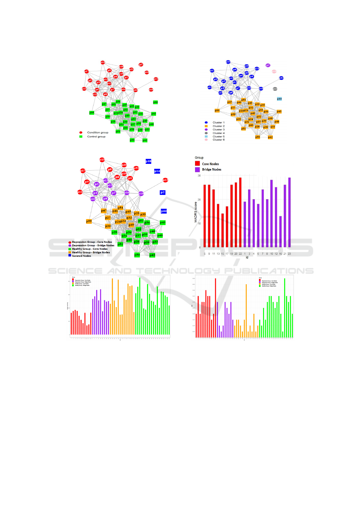
(a) Correlation Network graph. (b) Classiﬁcation.

(e) Mobility across different groups. (f) Age range across different groups.

Figure 2: Classiﬁcation and Severity estimation.

3 RESULTS

The study includes 55 participants of which 23 indi-

viduals belong to the condition group while 32 indi-

viduals belong to the control group. The novelty of

our approach is that we did not use the group label

(condition or control group) which is already present

in the dataset. We have built on the fact that the mobil-

ity of the condition group is lower and distinguishable

than the control group. Furthermore, we have utilized

graph properties in order to estimate the severity of

the depression. The results of our experiments are de-

scribed in the following sections.

3.1 Classiﬁcation

In the context of this article, the main aim of the clas-

siﬁcation task is to identify the subgroups that are in-

HEALTHINF 2023 - 16th International Conference on Health Informatics

420

herently present in the population. The classiﬁcation

task is performed in two stages. In the ﬁrst stage, a

correlation network is constructed as shown in Fig

.2(a), by incorporating 48 features derived in the ear-

lier step and by using a predeﬁned threshold T of

0.7. In the second stage, a clustering algorithm is em-

ployed to bring out the inherent clusters from the cor-

relation network. We have employed the MCL algo-

rithm to highlight the clusters in the graph network as

depicted in Fig. 2(b). The graph displayed in Fig.2(b)

demonstrates that two subgroups (condition and con-

trol) were fairly separated and established as sepa-

rate communities (clusters). Although we have not

used labels for classiﬁcation, we are referring to the

class label for the sake of accuracy estimation. Apart

from the isolated nodes, p1 through p23 which are

marked in blue belong to the condition group while

p24 through p55 which are marked in orange belong

to the control group.

3.2 Severity Estimation

The classiﬁcation task identiﬁed two major subgroups

as shown in Fig.2(b) . One of the subgroups is the

condition group while the other is the control group.

Since all the subjects belonging to the control group

are healthy and not diagnosed with depression, ill-

ness severity has been estimated only for the con-

dition group (p1 through p23). The DSS index is

measured using equation 2 for each participant from

the condition group. By utilizing the severity estima-

tion procedure mentioned in Table 1, all the nodes in

the condition group are split up into core nodes and

bridge nodes as shown in Fig.2(c). we have computed

score for each person in control group and categorized

them into two groups as shown in Fig. 2(c). (orange

and green color nodes). However, the description and

interpretation of these nodes are out of the scope of

this document.

4 ROBUSTNESS ANALYSIS

This section describes the validation analysis per-

formed on the obtained results. This manuscript

presents results in two folds. First, classiﬁcation be-

tween condition and control group without utilizing

label. Second, severity estimation of the condition

group those who are suffering from a depressive dis-

order.

4.1 Robustness of Classiﬁcation

In traditional label-driven classiﬁcation tasks such as

supervised machine learning techniques, the outcome

is solely dependent on labels present in the dataset.

Therefore, the classiﬁcation results are subject to bias

because of the labels present in the dataset. Further-

more, in medical datasets, it is not practical to expect

a label for every observation as its high time intensive

and requires huge human effort. To mitigate this prob-

lem, our classiﬁcation task is data-driven rather than

label-driven. However, we use existing class labels to

analyze the robustness of our methodology. Table 2 il-

lustrates the performance of the classiﬁcation task by

comparing our outcome against the known label. The

above results demonstrate that none of the subjects

were misclassiﬁed. Apart from the two major groups

some participants got isolated and not connected to

the network. Out of 55 subjects under the study, 4 of

them are isolated.

4.2 Robustness of Severity Estimation

In this section, severity estimation results of the con-

dition group are validated against the clinical rating

scale which is already present in the dataset. The clas-

siﬁcation task identiﬁed 20 subjects belonging to the

condition group out of a total of 23 subjects. Then,

the severity estimation task divided them into two

categories as shown in Table 1. To validate our re-

sults from the clinical context, participants with high

severity of depression are expected to possess a high

MADRS score whereas subjects with low severity are

expected to have a low MADRS rating. According to

MADRS ratings shown in Fig.2(d), our results prove

that core nodes are rated with a low MADRS score

while bridge nodes are rated with a MADRS rating.

Furthermore, the results demonstrate that the likeli-

hood of a DSS index reﬂecting a clinical rating scale

such as MADRS is very high.

Table 2: Classiﬁed category vs dataset label.

Actual

group

Classiﬁed group

Condition Control Isolated Total

Condition 20 0 3 23

Control 0 31 1 32

Total 20 31 4 55

A Correlation Network Model for Analyzing Mobility Data in Depression Related Studies

421

5 DISCUSSION

This research aimed to build a computational model

which is driven by the mobility data instead of the

class label present in the dataset. Most of the previ-

ous studies utilized supervised machine learning algo-

rithms in which a classiﬁer is trained on the existing

data with a known class label then the trained model

will be used to predict future instances. The disad-

vantage of this approach is that the training step ex-

pects all the class labels to be present in the dataset. It

implies that the dataset must contain a label indicat-

ing the health status of the subject. However, in the

real world, it is a tedious job to append health status

to each observation. Furthermore, the model should

be able to produce useful results even though the la-

bels are not available in the dataset. Our current work

in this paper attempts to bridge this gap. Since our

model does not necessitate a label to be annotated for

each observation, it works only by including mobility

data.

We have designed this model in two stages. First,

a correlation network graph is constructed. Second,

the MCL algorithm is employed to detect communi-

ties in the graph. The correlation between each pair of

subjects is measured using the Pearson correlation co-

efﬁcient with respect to 48 features. The intuitive idea

behind the construction of a correlation network is

that if any two subjects are connected by an edge, then

they are correlated concerning their mobility data. In

other words, two subjects are connected by an edge if

they possess similar mobility composition. Since our

method is not machine learning based, we do not use a

confusion matrix as a method of ﬁnding the accuracy

metric. But cluster quality metrics such as modular-

ity can be used. Yet, a quality metric such as mod-

ularity does not make sense in the case of biomedi-

cal datasets. Therefore, we have validated our results

against the clinical score available in the dataset.

In addition to the classiﬁcation and severity esti-

mation, we have performed an enrichment analysis to

verify if there are common and distinguishable demo-

graphic properties between or within the subgroups.

Enrichment analysis is a powerful computation tool

that has been heavily used in biomedical informat-

ics. In the past, researchers have mainly used this

technique to interpret gene expression data and com-

pare groups that display similar biological parameters

(Mclean et al., 2016). In this study, we have compared

the age and average motor activity of each person con-

cerning between subgroups and within the subgroup.

The results of this analysis are shown in Fig.2(e) and

Fig.2(f). Enrichment analysis reveals some interest-

ing facts that are signiﬁcant to consider. For example,

most of the participants in the high depression sever-

ity zone are younger than the high severity zone. Con-

versely, the mobility proﬁles of high-depression zone

subjects are lower than low depression subjects.

6 LIMITATIONS AND FUTURE

WORK

The primary focus of this work is to identify differ-

ent subgroups that are inherently present in the data

by utilizing their mobility data. A methodology is

a data-driven approach rather than label-driven. Al-

though our results are promising, there are certain

limitations in this study. First, even though the cor-

relation between the DSS index and MADRS clini-

cal score is very high, it is not always true. In other

words, a few participants’ DSS index is not reﬂect-

ing the MADRS score. This might be because of the

fact that the MADRS score might be always an ac-

curate measure of depression especially when the pa-

tients are under antidepression medication treatment

(Montgomery and

Asberg, 1979). In addition to that,

in the medical domain, it is always not viable to get

100% accurate results. However, our model has been

proposed based on the mobility data rather than de-

pending on the feelings or experiences of the clini-

cian. Secondly, the dataset contains only 23 subjects

belonging to the depression group. We do not reject

the limitation of a limited sample. Nevertheless, our

future work is acquiring larger datasets that include

multiple psychological disorders such as depression,

and ADHD.

7 CONCLUSION

Depression is a serious mental health disorder that can

negatively impact a person’s daily routine and cause a

signiﬁcant reduction in life span. Prolonged diagnosis

can cause deterioration in the mental health condition

and eventually reduces the possibility of treating the

illness or limit its effectiveness. Unfortunately, there

is no objective clinical test that can detect depres-

sion disorder and estimate its severity level. Existing

clinical procedures are predominantly driven by clin-

ician observation and self-reporting symptoms from

the patient or his/her family members. Neverthe-

less, many researchers have developed several com-

putational methods to address the problem. However,

most of these approaches are supervised and driven by

class labels there are present in the dataset. Append-

ing a label for every observation takes huge human

HEALTHINF 2023 - 16th International Conference on Health Informatics

422

effort and is impractical in real-world scenarios.

In this study, we introduce a novel data-driven

computational method that can classify depression

and estimate its severity level without using a class la-

bel. The proposed model is motivated by the fact that

reduced mobility is an early indication of depression.

At ﬁrst, a graph-based correlation network is con-

structed using the mobility data collected from wear-

able sensors and employing a clustering algorithm to

extract strongly connected communities (clusters) in

the graph. The advantage of employing the correla-

tion network model is that its underlying graph inher-

ently possesses the potential communities, and they

can be identiﬁed by s suitable community detection

clustering algorithm such as MCL. The obtained net-

work also has several graph-theoretic properties that

can be utilized to further analyze the mobility data.

Taking advantage of such properties, we have devel-

oped a new metric, Depression Severity Score index

(DSS), by using graph metrics including inter and

intra-cluster density. The obtained results demon-

strate that the correlation between measured DSS and

clinical depression rating score is high. We envision

that DSS can be used as a supplementary tool for clin-

icians and healthcare professionals in obtaining ob-

jective diagnostic assessment.

REFERENCES

Benesty, J., Chen, J., Huang, Y., and Cohen, I. (2009).

Pearson correlation coefﬁcient. In Noise reduction in

speech processing, pages 1–4. Springer.

Bondy, J. A., Murty, U. S. R., et al. (1976). Graph theory

with applications, volume 290. Macmillan London.

Cai, B.-J., Wang, H.-Y., Zheng, H.-R., and Wang, H. (2010).

Evaluation repeated random walks in community de-

tection of social networks. In 2010 International Con-

ference on Machine Learning and Cybernetics, vol-

ume 4, pages 1849–1854. IEEE.

Emmons, S., Kobourov, S., Gallant, M., and B

orner, K.

(2016). Analysis of network clustering algorithms

and cluster quality metrics at scale. PloS one,

11(7):e0159161.

Garcia-Ceja, E., Riegler, M., Jakobsen, P., Tørresen, J.,

Nordgreen, T., Oedegaard, K. J., and Fasmer, O. B.

(2018). Depresjon: a motor activity database of de-

pression episodes in unipolar and bipolar patients. In

Proceedings of the 9th ACM multimedia systems con-

ference, pages 472–477.

Li, Y., Babcock, S. E., Stewart, S. L., Hirdes, J. P., and

Schwean, V. L. (2021). Psychometric evaluation of

the depressive severity index (dsi) among children and

youth using the interrai child and youth mental health

(chymh) assessment tool. In Child & Youth Care Fo-

rum, volume 50, pages 611–630. Springer.

Mathers, C. D. and Loncar, D. (2006). Projections of global

mortality and burden of disease from 2002 to 2030.

PLoS medicine, 3(11):e442.

Mazza, M. G., De Lorenzo, R., Conte, C., Poletti, S., Vai,

B., Bollettini, I., Melloni, E. M. T., Furlan, R., Ciceri,

F., Rovere-Querini, P., et al. (2020). Anxiety and de-

pression in covid-19 survivors: Role of inﬂammatory

and clinical predictors. Brain, behavior, and immu-

nity, 89:594–600.

Mclean, C., He, X., Simpson, I. T., and Armstrong, D. J.

(2016). Improved functional enrichment analysis of

biological networks using scalable modularity based

clustering. Journal of Proteomics & Bioinformatics,

9(1):9–18.

Montgomery, S. A. and

Asberg, M. (1979). A new depres-

sion scale designed to be sensitive to change. The

British journal of psychiatry, 134(4):382–389.

The National Institute of Mental Health (NIMH) (2021).

Depression. [Online; accessed 8-August-2021].

Thelagathoti, R. and Ali, H. (2022a). A population analysis

approach using mobility data and correlation networks

for depression episodes detection. Ann Depress Anxi-

ety, 9(1):1112.

Thelagathoti, R. K. and Ali, H. H. (2022b). The compari-

son of various correlation network models in studying

mobility data for the analysis of depression episodes.

In BIOSIGNALS, pages 200–207.

Williams, J. B. (1988). A structured interview guide for the

hamilton depression rating scale. Archives of general

psychiatry, 45(8):742–747.

A Correlation Network Model for Analyzing Mobility Data in Depression Related Studies

423