Step Towards Generalization: Fault Classification in Multivariate

High-Frequency Data from Different Operating Regimes of

Hydraulic Rock Drill System

Nagi Reddy, Ashit Gupta, Gauri Dhande and Vijaykumar Pasupureddy

Center for Intelligent Power, Eaton India Innovation Center, Pune, India

Keywords: Industrial Application, Fast Oscillating Hydraulic Rock Drill, Fault Classification, ResNet.

Abstract: Hydraulic rock drills operate under harsh environments of excessive humidity and vibrations. In operation,

the fundamental machine frequency is hampered by various loading disturbances created by the pressure

waves generated during the rock drill application, which initiates faults at different times during a complete

cycle of rock drilling. These faults include failure of internal parts, excessive channel openings and damaged

parts, causing enough non-linearity in the pressure data generated. A fault in such machinery can multiply

quite rapidly, leading to accidents like complete failure of the equipment and loss of life. Therefore, it is

crucial to classify the fault and inform the operator of it. The fault classification challenge escalates further

when the rock drill operates on previously unknown operating conditions. In the present work, we compare

the performance of deep learning models like Long short-term memory, Convolutional Neural Network, and

Residual Network to classify faults, whose signature is recorded in data generated at a frequency of 50kHz

when a rock drill is in operation. We also demonstrate how the accuracy of models vary when the models are

tested on unseen operating conditions. An overall analysis is provided to generalize a model for fault

classification in industrial applications over contrasting operating conditions.

1 INTRODUCTION

Hydraulic rock drills have a wide range of

applications in various industries, such as mining,

rock excavation projects, highway tunnels, and

railways, due to their high precision, cleanliness, and

safety (Ma et al., 2019). Modern rock drills are

generally mounted on vehicles and their mechanism

uses pneumatics or hydraulics (Jakobsson et al,

2022). Hydraulic rock drills are used to fracture huge

rocks and concrete structures by applying pressure

through continuous impact & rotation, with a force of

around 600kN. The repetitive impact of piston makes

the machine vulnerable to different faults.

Classification of faults is crucial to ensure safety and

maintain high maintenance standards. Different

operating regimes recorded different signatures of

fault, making the classification problem more

challenging. Therefore, a model that guarantees that

a fault is captured and categorizes it appropriately is

needed.

Due to high reliability, robustness, and low cost,

only pressure sensors are mounted on hydraulic rock

drills. Pressure waves generated are recorded on these

sensors at a frequency as high as 50kHz. These

pressure signals are recorded at the inlet fitting called

percussion pressure (P

), damper pressure inside the

outer chamber (P

din

), and pressure in the volume

behind the piston (P

). The magnitude and phase of

these pressure signals depend on the impact of the

drill on the rock or sudden valve openings (Jakobsson

et al., 2022). The pressure is recorded for a certain

period depending on the overall operation time of the

hydraulic rock drill or the occurrence of an

unforeseen event such as faults. The measured signal

is periodic in nature, typically, governed by a

sequence of valve openings at different times, making

it difficult to view the signal as a superposition of

similar wave occurrences in the past. Additionally,

these events correlate to fault occurrences, and they

vary with a change in test setup or change in operating

conditions, therefore, making it difficult to spot the

occurrence of individual events at such a high

frequency of event generation.

Hydraulic rock drill operates under high-

performance demands in harsh environments

856

Reddy, N., Gupta, A., Dhande, G. and Pasupureddy, V.

Step Towards Generalization: Fault Classiﬁcation in Multivariate High-Frequency Data from Different Operating Regimes of Hydraulic Rock Drill System.

DOI: 10.5220/0011676100003411

In Proceedings of the 12th International Conference on Pattern Recognition Applications and Methods (ICPRAM 2023), pages 856-863

ISBN: 978-989-758-626-2; ISSN: 2184-4313

 2023 by SCITEPRESS – Science and Technology Publications, Lda. Under CC license (CC BY-NC-ND 4.0)

subjected to excessive humidity and vibrations

(Jakobsson et al., 2022). In operation, the

fundamental machine frequency is hampered by

various loading disturbances created by the pressure

waves, generated during the rock drill application.

This initiates faults at different times during a

complete cycle of rock drilling. These faults include

failure of internal parts, excessive channel openings,

and damaged parts. The fault classification challenge

escalates further when the hydraulic rock drill

operates in an unseen test environment. Table 1

represents 11 types of faults occurring in hydraulic

rock drills in operation.

Table 1: Fault Classes for a hydraulic rock drill.

Class

Numbe

Class

Code

Class Description

Fault 0 NF No fault

Fault 1 T Thicker drill Steel

Fault 2 A Leakage from high-pressure

channel to low-

ressure channel

Fault 3 B Leakage from the control channel

the to return channel

Fault 4 R Damaged return accumulato

Fault 5 S Longer drill steel

Fault 6 D The damper orifice is larger than

usual

Fault 7 Q Low flow to the damper circuit

Fault 8 V Valve damage

Fault 9 O The orifice on control line outlet

larger than usual

Fault 10 C The charge level in high-pressure

accumulator is low

Research in classification algorithms based on

machine learning, deep learning, or symbolic learning

has certainly taken up a developmental pace since the

last decade (Gupta et al., 2021). Every year work on

new classification approaches has been proposed that

work extremely well on benchmark datasets provided

under the UCR archive for numerous industrial

applications and academic interests (Dau et al., 2019).

Few of the frequently tested algorithms for such tasks

are LSTMs, CNNs, and transformers. with their

variants including architecture changes or ensemble

strategies (Gupta et al. 2021).

Researchers have proposed some related work on

fault classification using sensor data with time series

models or other deep learning frameworks. Sun et al.

(2020) have proposed a CNN-based framework by

using univariate sensor data from a hydrogen sensor.

They have also proposed the usage of random forest

as a bagging algorithm to generalize their model.

Although they were able to achieve an accuracy of

100% for 6 faults, the faults considered had very

different signatures, and the faults that possess signals

closer to the base faults were considered as future

work (Sun et al., 2020). Few researchers have used

deep convolutional neural networks (DCNN) to

identify faults in gearbox sensor data (Jing et al.,

2017). They transformed the data into 3 fusion levels

and were able to achieve high accuracies after

transformation. However, the data present in training,

validation, and test sets were taken up from the same

test facility. They did not have any separate data from

different test setups or different operating conditions.

Researchers have also experimented with 3 types of

datasets of motor bearing with 2 faults outer ring and

inner ring faults using a Transfer Convolutional

Neural Network (Wen et al., 2020). They also divided

the data into train, validation, and test from the same

datasets and provided k-fold validation. Both the

aforementioned works make it difficult to scale up the

model for different test facilities or operating

conditions. Zhang et al. (2021) have used a hybrid

attention Resnet to train a model for fault diagnosis of

wind turbine gearbox. The present work is inspired by

their idea of fault diagnosis, and we propose the use

of Resnet for generalizing a model for multiple

operating regimes.

Jakobsson et al. (2022), have also proposed a time

series-based approach for fault classification in

hydraulic rock drill operations. They have employed

Dynamic Time Warping (DTW) with its several

variations. They have used only one pressure sensor

(percussion pressure) and have reported the best

accuracy of 73% on the test dataset (i.e., changing

operating conditions). The hypothesis followed

requires that signatures of one fault would always

follow the same trend in any operating condition and

the change would only be compromised in the phase

difference, where the DTW algorithm with its

variants can help. In the present work, we employ

several deep learning-based approaches to capture the

spatial and temporal patterns in the multivariate data

and discuss the best model that can be deployed.

The present work proposes the development of

algorithms where operating regimes of industrial data

changes in relation to the necessary application, as a

result, similar trends are unseen while model training.

This work intends to obtain a generic model for

deployment with an assumption that data available for

training is scarce and the test operating conditions are

completely unseen by the model. The contribution of

this work provides an approach for solving industrial

problems with changing operating regimes,

decomposing domains based on available data, and

lastly, selecting the best model for deployment.

Step Towards Generalization: Fault Classiﬁcation in Multivariate High-Frequency Data from Different Operating Regimes of Hydraulic

Rock Drill System

857

The paper is organized as follows: Section 1

describes the problem statement, industrial standards,

related work, and the identified gaps. Section 2

describes the data source and descriptive study.

Section 3 describes the architectures of the algorithms

used. Section 4 presents the methodology followed to

select the best model. Section 5 presents the key

results and provides relevant discussion around them.

Lastly, section 6 summarizes the approach & results

and provides concluding remarks.

2 DATA DESCRIPTION

The hydraulic rock drill system in consideration uses

3 sensors, mounted at different locations on the drill,

recording pressure at a frequency of 50kHz. The

pressure data used for analysis is generated in a test

facility where the faults are induced in the system for

different operating conditions (Jakobsson et al.,

2022). Multiple instances are captured in the test

facility by changing the operating conditions of the

hydraulic rock drill. The test facility is kept as close

to real-world scenarios, where drilling usually takes

place. Any modifications to percussion pressure (P1)

and feed force (P2) have a significant impact on how

hydraulic rock drill operates. Experiments have been

conducted by changing feed force and percussion

pressure and as a result pressure variations are

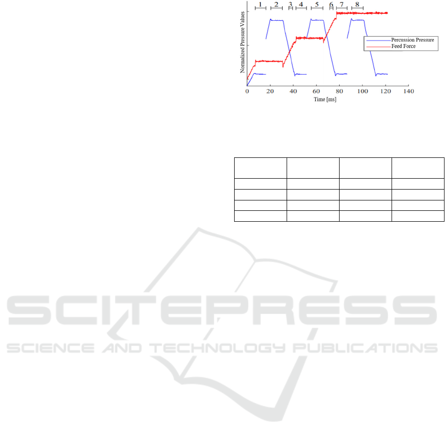
recorded on the 3 pressure sensors. Figure 1 illustrates

the changing operating conditions with respect to

controllable variables (P1 and P2). Additionally,

changes in ambient conditions and the direction of

drilling are a few uncontrollable parameters that alter

the pressure signal recordings, thereby making the

fault classification task complex.

Figure 1 illustrates eight distinct operational

regimes that have been recorded based on the

outcomes of trials carried out in the testing facility.

Each of the operating regimes provided has a

different set of P1-P2 values. Table 2 provides the

number of observations captured in each of the

operational regimes. The fault classes were evenly

separated in all the regimes.

Figure 3 illustrates how the same fault differs

under several operational regimes. The x-axis in the

figure represents the time in milliseconds and the y-

axis represent the P

, P

din,

and P

for a single fault.

From the exploratory analysis in figure 3, it can be

noted that a single fault's patterns alter over various

operating regimes and cannot be superimposed on

one another. Therefore, advanced algorithms are

needed to classify faults with high accuracy.

Figure 1: Percussion pressure & feed force variation for all

8 operating regimes (Jakobsson et al., 2022).

Table 2: Regime-wise data samples available.

Regime ID Number of

sam

les

Regime ID Number of

sam

les

Regime 1 7311 Regime 5 7977

Regime 2 7867 Regime 6 3293

Regime 3 3184 Regime 7 7935

ime 4 7597 Re

ime 8 8461

3 NETWORK ARCHITECTURES

We tested 3 deep learning architectures to provide the

best possible accuracy even when the operating

conditions change. We consider the work done by

Jakobsson et al. (2022), as a baseline and explore the

outcomes from deep learning architectures. Each of

the network architectures is built using the functional

API in TensorFlow 2.0 (Abadi et al., 2016)

3.1 Long Short-Term Memory

Long short-term memory (LSTM) is a sequential

deep learning algorithm introduced to overcome the

vanishing gradients problems usually noticed in

Recurrent Neural Networks (RNN) (Hochreiter et al.,

1997). LSTM networks are known to provide

excellent results when the features in the data have

temporal dependencies. In the past LSTMs have been

successful in industrial applications such as problems

with classification applications, prediction

applications, anomaly detection, forecasting

applications, etc. (Balouji et al., 2018, Gupta et al.,

2022). The predictions from an LSTM model are

controlled by 3 control gates; an input/update gate,

forget gate, and an output gate. The previous hidden

state and the current input are fed to the input/update

gate, while forget gate controls the amount of

previous information to be passed to the next cell

state, and lastly, the output gate decides the final state

of the cell. Figure 4 presents the architecture of the

network used in the current study.

ICPRAM 2023 - 12th International Conference on Pattern Recognition Applications and Methods

858

Figure 2: (a) Normalized damper pressure inside the outer chamber, (b) Normalized pressure in the volume behind the piston,

and (c) Normalized percussion pressure at inlet fittings vs time in milliseconds.

Figure 3: Normalized damper pressure, Normalized pressure in the volume behind the piston & normalized percussion

pressure showing the variation in fault signatures in all operating regimes for different cases. 1. No-fault scenario, 2. Thicker

drill steel fault, and 3. Leakage from high pressure to low pressure challenge fault.

Step Towards Generalization: Fault Classiﬁcation in Multivariate High-Frequency Data from Different Operating Regimes of Hydraulic

Rock Drill System

859

The model architecture is illustrated in figure 4.

The model consists of 2 LSTM layers of 80 and 60

LSTM units, with an activation function as tanh. The

2 LSTM layers are followed by 3 dense layers

consisting of 50, 25, and 11 dense units respectively.

The first 2 dense layers are provided with a relu

activation function while the last output layer has a

softmax activation function. The tuning of the

hyperparameters is carried out using a random search

method. The model is trained over 260 epochs with a

batch size of 32 and a learning rate of 1e-4.

Figure 4: LSTM architecture.

3.2 Convolutional Neural Networks

Convolutional neural networks have shown great

promise in a variety of applications, especially in

image-based datasets for applications such as image

classification, image detection etc. (Aloysius et al.,

2017). The main difference between a neural network

and the convolutional neural network is in the

selective connection of neurons between hidden

layers. Because of this sparse connectivity, a CNN

model can learn spatial features implicitly. CNN

model uses a convolutional operator resulting in

neurons sharing weights, thereby, reducing the

complexity of the model by decreasing the number of

trainable weights. Recently, the performance of

CNN-based architectures has shown promise in

industrial applications such as fault diagnosis,

classification, and prediction (Jiao et al, 2020).

The CNN model architecture is illustrated in

figure 5. The model consists of 4 CNN-1D layers with

128, 256, 128, and 128 filters respectively. The filter

size and activation functions used are shown in figure

5. The 4 CNN layers are followed by 2 dense layers

(including the output layer) with the number of

neurons in each layer equal to 20 and 11. A batch size

of 8 with a learning rate of 0.00001 is used to train the

model for 100 epochs.

Figure 5: CNN architecture.

3.3 Residual Networks (ResNets)

ResNets were introduced to improve the performance

of deep neural networks in Image classification (He

et al., 2016). The introduction of skip connections

between residual blocks enabled the gradient flow to

the bottom layers. Figure 6 shows an image of such

residual block connection. ResNet achieved state-of-

the-art performance on ImageNet, COCO datasets

etc. Similarly, it has shown optimal performance in

time series Datasets in UCR (Dau et al., 2019).

Figure 6: Connection within a ResNet.

The customized ResNet architecture used in this

study is illustrated in figure 7. The network consists

of 3 Residual blocks with convolutional filters

64,128, and 128 respectively. Each Residual block

consists of 3 convolutional 1-D with filter sizes

{5,3,1}, followed by batch normalization with

activation function relu. These residual blocks are

followed by a global average pooling layer and an

output layer with 11 neurons. A batch size of 8 with a

learning rate of 0.00001 is used to train the model for

100 epochs.

All the models are trained on a GPU machine with

specifications: NVIDIA RTX A4000 processor on

ubuntu 22.04 version on a 64-bit operating system,

with 48 GB RAM.

ICPRAM 2023 - 12th International Conference on Pattern Recognition Applications and Methods

860

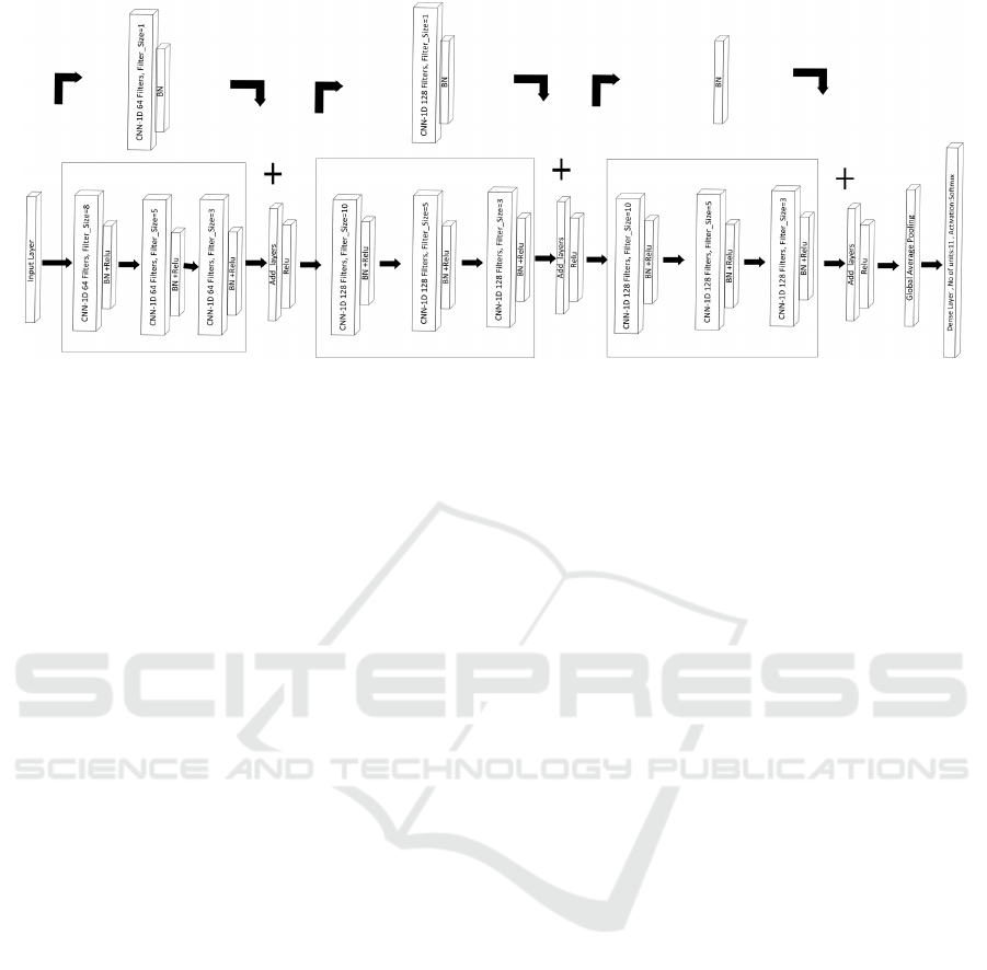
Figure 7: Resnet architecture.

4 METHODOLOGY

Figure 3 illustrates the change in operating regimes

with respect to the change in P1 and P2 for a hydraulic

rock drill system. Jakobsson et al. have also

mentioned that changing feed force (P2) majorly

affects the fault signature which lead to inaccuracy in

their model. Therefore, it is important to develop a

framework where the accuracy of the model is not

hampered by changing operating conditions.

Considering generalization to be of paramount

importance we formulated 3 parallels to build models

as accurate as possible that works even in changing

operating conditions.

4.1 Enclosed Operating Regime

Prediction

Different operating regimes are generated by varying

both the parameters (P1 & P2), which are shown as 1-

8 numeric values in figure 1. These operating regimes

indicate the real-time working conditions, such as the

operating regime may imply straightforward

drilling circumstances in delicate rocks, whilst the 8

operating regime may indicate some complex rock

excavation in coal mines. In the enclosed operating

regime prediction approach, data from one operating

regime is split into train, validation, and test dataset

in the ratio 70:15:15. Deep learning architectures

presented in section 3 are trained, and their

performances are recorded. The 15% test data and

adjacent regime data are used to evaluate the

performance of all models. The latter enables the

selection of best models performing well not only on

the base operating regime (training data operating

regime) but also on an unseen operating regime.

As an example, 70% of data from 1

operating regime

is used to train the models. These models are then

used to predict faults on samples from 2

operating

regime only. This test is done on the adjacent regime

with respect to P2 so that model’s judgment makes

sense.

4.2 Intermediate Operating Regime

Prediction

In the intermediate operating regime prediction

approach, operating regimes 1,2,4,5, and 6 are used to

train a model, and the model’s performance is tested

on the 3

operating regime. In this method, the model

is trained from scratch from 1 boundary to another

while allowing a few operating circumstances for

testing in between, ensuring great performance on

intermediate unseen data.

4.3 Exterior Operating Regime

Prediction

Rock drill application involves crushing both soft and

hard rocks, requiring changes in feed force from as

low as 20kN to 600kN (Jakobsson et al, 2022). Since

there is such a large variation in force, many times

rock drill machines have not seen high-force tasks.

Safety being of utmost importance necessitates the

prediction and classification of a fault even if the

large feed force operating condition is not seen during

model training. Therefore, a model that can

accurately anticipate a class is needed for exterior

operating regime prediction approach.

Here, we use the training datasets 1, 2, 3, and 4

to train the CNN & Resnet models from scratch and

test the models on test datasets 5 & 6. Then, in order

Step Towards Generalization: Fault Classiﬁcation in Multivariate High-Frequency Data from Different Operating Regimes of Hydraulic

Rock Drill System

861

to generalize the model to any operating regime, the

model architecture with the highest accuracy in

exterior operating regime prediction would be

adopted. It would be trained on operating regimes 1,

2, 3, 4, 5 & 6 and tested on operating regimes 7 & 8.

5 RESULTS & DISCUSSIONS

Prior work done by Jakobsson et al. (2022) sets the

baseline for any model development, where

improvement in the results of fault classification

demands an increase in accuracy. They used Dynamic

Time Warping (DTW) and its derivatives to achieve

an accuracy of 100% on predictions in an enclosed

operating regime and reported 73% on any other

operating regime. In the present work, we consider

their achievements as the baseline and develop

models that work well not only on enclosed operating

regime data points but also on intermediate and

exterior operating regime data points.

Three types of base model architectures are used

to classify faults: LSTM, CNN, and ResNets. Each

model is randomly customized to produce the highest

test accuracy for each approach presented in section

4. The ResNet model is customized by changing the

skip connections in the architecture for the

classification problem under study. The time taken to

train, number of trainable parameters, and the results

are presented in Table 4.

Table 4 presents results for all three operating

regimes. First, all three models are tested on the

enclosed operating regime. Here, all the models are

trained on 70% of data from 1

operating regime and

are validated on 30% of data from the same regime.

All 3 algorithms predict the fault class with at least

98.32% accuracy in training data and at least 89%

accuracy in validation data. ResNets perform best

with 100% accuracy in both, while the performance

of LSTM-based model can be deemed as overfitted.

Although, the accuracy of prediction for all the

models is quite high on the data from the same

operating regime, but all models failed to produce

good accuracy when tested on data points from 2

operating regime. ResNets-based model generated

maximum accuracy equal to 42.48%, while the

LSTM-based model had the least accuracy equivalent

to 10.52%. This drop in accuracy can be attributed to

the unobserved operational condition of percussion

pressure (P1) by the models, resulting in the recording

of unseen pressure disturbances on the 3 pressure

sensors. Therefore, it can be concluded that models

require more knowledge of the operation of hydraulic

rock drills to generalize for any operating condition.

Second, we analyze models’ performance on the

intermediate operating regime. Here, all the models

are trained on 70% of the training data (operating

regimes: 1,2,4,5,6) and their predictions are validated

on 30% of unseen data from the same regimes, while

the data recorded in the 3

operating regime is

considered to be the test data. The accuracy of the

LSTM-based model dropped drastically for both

validation and test datasets. The drop in accuracy can

be attributed to the failure of LSTM networks to

classify on samples from extrapolated data, similar to

the results reported by Trask (Trask et al, 2018). On

the other hand, CNN & ResNet- based models were

able to capture faults perfectly.

Lastly, we examine the performance of CNN-

based and ResNet-based models on exterior operating

regimes. ResNet architecture provided the highest test

accuracy on operating regimes 5 & 6, equivalent to

98.61%. Moreover, the recall value on the fault is

generally considered a measure of safety for

equipment. Table 3 shows that none of the actual fault

cases are classified as healthy working conditions (no

fault class) of the equipment, resulting in a recall

value equivalent to 1 over fault. A high recall value is

generally considered as a safety measure for any

equipment in operation. Here, the recall value for the

ResNet model is equal to 1, hence satisfying the

safety criteria for such huge machinery.

Additionally, the model was also trained on

operating regimes 1,2,3,4,5, & 6 and tested on

operating regimes 7&8. ResNet model was able to

produce an accuracy of 98.09%, which ensures the

stability of the model in varying operating conditions.

Therefore, it can be noted that ResNet model with the

proposed architecture, trained with the least amount

of time taken, is a better measure of accuracy and

safety for the equipment under study.

Table 3: Confusion matrix for ResNet on 5&6 operating

regime for fault & no faults scenario.

Predicted

Actual

Fault No-Fault

Fault 10259 0

No-Fault 27 984

6 CONCLUSIONS

In this paper the generalized approach for the Fault

Classification over different operating regimes of

hydraulic rock drill system has been presented. The

outcomes of 3 different model architectures built

using LSTM, CNN, and ResNets base layers were

ICPRAM 2023 - 12th International Conference on Pattern Recognition Applications and Methods

862

compared for each region. An accuracy of 100% was

produced on previously unknown intermediate

regimes by CNN & ResNet. On unobserved exterior

regimes, the proposed ResNet architecture

demonstrated the best accuracy of 98.61% and

98.09%. Furthermore, classification done using

Resnet model produced a recall value of 1 over faults,

guaranteeing the safety of operation in such complex

machinery. Therefore, it can be concluded that the

proposed ResNet architecture is the generalized

model for fault classification in any operating regime

of a hydraulic rock drill setup.

REFERENCES

Abadi, M., Agarwal, A., Barham, P., Brevdo, E., Chen, Z.,

Citro, C., ... & Zheng, X. (2016). Tensorflow: Large-

scale machine learning on heterogeneous distributed

systems. arXiv preprint arXiv:1603.04467.

Aloysius, N., & Geetha, M. (2017, April). A review on deep

convolutional neural networks. In ICCSP (pp. 0588-

0592). IEEE.

Balouji, E., Gu, I. Y., Bollen, M. H., Bagheri, A., & Nazari,

M. (2018, May). A LSTM-based deep learning method

with application to voltage dip classification. In 2018

18th ICHQP (pp. 1-5). IEEE.

Chen, X., Zhang, B. and Gao, D. (2021). Bearing fault

diagnosis base on multi-scale CNN and LSTM model. In

Journal of Intelligent Manufacturing, 32(4), pp.971-987.

Dau, H. A., Bagnall, A., Kamgar, K., Yeh, C. C. M., Zhu,

Y., Gharghabi, S., ... & Keogh, E. (2019). The UCR

time series archive. In IEEE/CAA Journal of

Automatica Sinica, 6(6), 1293-1305.

Gupta, A., Jadhav, V., Patil, M., Deodhar, A., & Runkana,

V. (2021, July). Forecasting of Fouling in Air Pre-

Heaters Through Deep Learning. In ASME Power

Conference (Vol. 85109, p. V001T01A002). American

Society of Mechanical Engineers.

Gupta, A., Masampally, V. S., Jadhav, V., Deodhar, A., &

Runkana, V. (2021, January). Supervised Operational

Change Point Detection using Ensemble Long-Short

Term Memory in a Multicomponent Industrial System.

In 2021 SAMI (pp. 000135-000141). IEEE.

Hochreiter, S., & Schmidhuber, J. (1997). Long short-term

memory. Neural computation, 9(8), 1735-1780.

He, K., Zhang, X., Ren, S., & Sun, J. (2016). Deep residual

learning for image recognition. In Proceedings of the

IEEE conference on computer vision and pattern

recognition (pp. 770-778).

Ismail Fawaz, H., Forestier, G., Weber, J., Idoumghar, L.,

& Muller, P. A. (2019). Deep learning for time series

classification: a review. Data mining and knowledge

discovery, 33(4), 917-963.

Jakobsson, E., (2022). Condition Monitoring in Mobile

Mining Machinery., Doctoral dissertation, Linköping

University Electronic Press.

Jakobsson, E., Frisk, E., Krysander, M. and Pettersson, R..,

(2022). Time Series Fault Classification for Wave

Propagation Systems with Sparse Fault Data. arXiv

preprint arXiv:2203.16121.

Jiao, J., Zhao, M., Lin, J., & Liang, K. (2020). A

comprehensive review on convolutional neural network

in machine fault diagnosis. Neurocomputing, 417, 36-63.

Jing, L., Wang, T., Zhao, M. and Wang, P. (2017). An

adaptive multi-sensor data fusion method based on deep

convolutional neural networks for fault diagnosis of

planetary gearbox. Sensors, 17(2), p.414.

Ma, W., Geng, X., Jia, C., Gao, L., Liu, Y. and Tian, X.

(2019). Percussion characteristic analysis for hydraulic

rock drill with no constant-pressurized chamber

through numerical simulation and experiment.

In Advances in Mechanical Engineering, 11(4),

p.1687814019841486.

Sun, Y., Zhang, H., Zhao, T., Zou, Z., Shen, B. and Yang,

L., (2020). A new convolutional neural network with

random forest method for hydrogen sensor fault

diagnosis. IEEE Access, 8, pp.85421-85430.

Trask, A., Hill, F., Reed, S. E., Rae, J., Dyer, C., & Blunsom,

P. (2018). Neural arithmetic logic units. Advances in

neural information processing systems, 31.

Wen, L., Li, X. and Gao, L. (2020). A transfer

convolutional neural network for fault diagnosis based

on ResNet-50. Neural Computing and Applications,

32(10), pp.6111-6124.

Zhang, K., Tang, B., Deng, L., & Liu, X. (2021). A hybrid

attention improved ResNet based fault diagnosis

method of wind turbines gearbox. Measurement, 179,

109491.

Table 4: Classification accuracy for all the models in all operating regimes.

S.No Regime Model base

Laye

# Trainable

Parameters

Training

Time

Training

Accuracy (%)

Validation

Accuracy (%)

Test

Accuracy (%)

1 Enclosed

Operating Regime

LSTM 65311 ~4 hrs 98.32 89.1 10.52

2 CNN 987291 ~1.5 hrs 100 99.2 28.62

3 ResNet 506571 ~1 h

100 100 42.48

4 Intermediate

Operating Regime

LSTM 65311 ~4hrs 85.37 63.78 41.21

5 CNN 987291 ~1.5 hrs 100 100 100

6 ResNet 506571 ~1 h

100 100 100

7 Exterior Operating

Regime

LSTM 65311 ~4 hrs 81.21 41.35 22.94

8 CNN 987291 ~1.5 hrs 100 100 91.25

9 ResNet 506571 ~1 h

100 100 98.61

Step Towards Generalization: Fault Classiﬁcation in Multivariate High-Frequency Data from Different Operating Regimes of Hydraulic

Rock Drill System

863