Uncertainty-Aware DPP Sampling for Active Learning
Robby Neven
a
and Toon Goedem
´
e
b
PSI-EAVISE, KU Leuven, Jan Pieter De Nayerlaan, Sint-Katelijne-Waver, Belgium
Keywords:
Deep Learning, Machine Learning, Computer Vision, Active Learning.
Abstract:
Recently, deep learning approaches excel in important computer vision tasks like classification and segmen-
tation. The downside, however, is that they are very data hungry, which is very costly. One way to address
this issue is by using active learning: only label and train on diverse and informative data points, not wasting
any effort on redundant data. While recent active learning approaches have difficulty combining diversity and
informativeness, we propose a sampling technique which efficiently combines these two metrics into a single
algorithm. This is achieved by adapting a Determinantal Point Process to also consider model uncertainty.
We first show competitive results on the academic classification datasets CIFAR10 and CalTech101, and the
CityScapes segmentation task. To further increase the performance of our sampler on segmentation tasks,
we extend our method to a patch-based active learning approach, improving the performance by not wasting
labelling effort on redundant image regions. Lastly, we demonstrate our method on a more challenging real-
world industrial use-case, segmenting defects in steel sheet material, which greatly benefits from an active
learning approach due to a vast amount of redundant data, and show promising results.
1 INTRODUCTION
While recent works on deep neural networks excel
in computer vision tasks like classification, detection
and semantic segmentation, the downside of these
methods is that they are very data hungry. For each
algorithm to perform best, an abundance of highly-
detailed, labeled data samples are needed to train
these networks, which is very costly. Besides of a
high labeling cost, many industrial applications also
require expert knowledge to acquire and correctly la-
bel samples, which can severely slow down the time
to production.
Many recent works have pointed out this prob-
lem and have approached it in multiple ways. To
reduce the data need, approaches such as few shot
learning, semi-supervised and self-supervised meth-
ods have been able to prove their worth in effec-
tively training a network by drastically reducing the
labelling effort.
One other approach is active learning. In contrast
to training a network on a large dataset, the goal of
active learning is to train the model on a well-chosen,
smaller subset of highly informative and diverse data
points without reducing performance. Active learn-
ing is based on the idea that standard datasets con-
a
https://orcid.org/0000-0003-0857-1310
b
https://orcid.org/0000-0002-7477-8961
sists of many redundant data points which are similar
in the amount of information they are carrying and
can be represented by a more compact dataset. While
training on a smaller, more compact dataset clearly
reduces the amount of training time, it not only drasti-
cally reduces the amount of labeling effort, but more-
over, the model’s optimization is more efficient since
an active learning algorithm constructs a dataset by
actively searching for highly informative and diverse
data points.
There are two main approaches of active learn-
ing: pool-based versus stream based active learning.
In this work, we mainly focus on pool-based active
learning, which starts with a large unlabeled data pool
from which the active learning algorithm iteratively
selects a smaller subset to manually label and train
the main task model on. By iteratively sampling and
training on small batches, the sampling algorithm can
use the model’s performance to focus on more diffi-
cult (informative) training samples and ignore redun-
dant samples from the large data pool.
To be effective, active learning needs to priori-
tize samples based on their diversity and informative-
ness. Diversity focuses on samples which are visually
dissimilar, while informativeness is a score to iden-
tify how much information this sample could bring to
the next iteration of the model. While diversity con-
structs a visually diverse dataset, informativeness is
Neven, R. and Goedemé, T.
Uncertainty-Aware DPP Sampling for Active Learning.
DOI: 10.5220/0011680100003417
In Proceedings of the 18th International Joint Conference on Computer Vision, Imaging and Computer Graphics Theory and Applications (VISIGRAPP 2023) - Volume 4: VISAPP, pages
95-104
ISBN: 978-989-758-634-7; ISSN: 2184-4321
Copyright
c
 2023 by SCITEPRESS – Science and Technology Publications, Lda. Under CC license (CC BY-NC-ND 4.0)
95

an even important metric since this is mostly based
on the model’s uncertainty and indicates any knowl-
edge gaps the model still has. While recent works
mainly focus on either diversity or informativeness,
in this paper, we leveraged both metrics in our active
learning setup sampling technique to sample the most
efficient data points in each active learning step.
In this work, we propose a new pool-based ac-
tive learning algorithm which leverages both diver-
sity and informativeness by combining the model’s
uncertainty with a Determinantal point process (DPP)
(Kulesza, 2012). A DPP is a point process based on
negative correlations between data points, which can
be leveraged to enforce diversity when used on mean-
ingful sample representations. While sampling a sub-
set from the DPP enforces diversity, after each active
learning step, we can evaluate the model’s uncertainty
on each data point, indicating a measure of informa-
tiveness. Having this informative score, we adapted
the DPP’s sampling to incorporate this score, which
influences the negative correlations between similar
data points. While a DPP inherently only focuses on
diversity, it now focuses both on diverse and informa-
tive data points.
We tested our method on two important visual
tasks: image classification and semantic segmenta-
tion. For the classification task we used the popular
CIFAR10 and CalTech101 datasets, while for the seg-
mentation task we focused on the autonomous driving
dataset CityScapes. For each task, we showed the ef-
fectiveness of our method and compared against other
recent active learning approaches. For the segmenta-
tion task, we also extended our sampling method to
a patch based approach. While sampling whole im-
ages can be effective, for some datasets, there is re-
dundancy within images, which can be excluded by
actively searching for diverse and informative patches
within images. This method spends the labeling effort
in a more efficient manner throughout the dataset, re-
sulting in a further increased performance.
To conclude, the main contributions of this paper
are:
• We propose a new active learning algorithm
which combines a Determinantal Point Process
with model uncertainty to simultaneously focus
on diversity and informativeness.
• We demonstrate the superiority of our approach
with respect to other state-of-the-art methods on
two important computer vision tasks, including
classification and segmentation.
• We extend our active learning method for segmen-
tation to a patch based approach, which further in-
creases the performance by spending the labelling
budget in a more efficient manner throughout the
dataset.
2 RELATED WORK
As we have already mentioned, deep neural net-
works perform best when combined with abundant,
highly detailed annotated datasets. Therefore, many
works on active learning tried to approach the prob-
lem by constructing these datasets as efficient as pos-
sible without wasting any labeling budget. The two
main active learning approaches are pool-based ver-
sus stream based. The latter deals with a constant
data stream from which the active learning algorithm
selects samples in an online manner. On the other
hand, pool-based active learning starts from an unla-
beled data pool, from which the active learning algo-
rithm iteratively samples subsets to train the model
on. In this work, we will only focus on pool-based
active learning.
Early works on active learning focused on in-
formation theoretical approaches (MacKay, 1992),
ensemble methods (Freund et al., 1995; McCallum
and Nigam, 1998), uncertainty based methods (Joshi
et al., 2009; Tong and Koller, 2002) and Bayesian ac-
tive learning methods (Kapoor et al., 2007). While
these methods have proven their worth for smaller
scale datasets, current large-scale datasets for deep
learning require different approaches.
More recent work on active learning for large-
scale datasets can be divided into two main groups:
informativeness versus diversity. Methods focussing
on diversity try to understand the distribution of the
unlabeled data and try to sample a representative sub-
set. One approach (Sener and Savarese, 2017) used
a core-set sampling method to reduce the dataset into
high diverse data points based on a CNN-based fea-
ture distribution. Other approaches try to model the
distribution of a labeled dataset using a variational
auto encoder (Sinha et al., 2019) to select new sam-
ples from an unlabeled dataset. The VAE models the
distribution of a pre-labeled subset and trains a dis-
criminator on both the labeled and unlabeled set to
identify a data point as labeled or not. This will ac-
tively search for samples which are out of distribution
of the labeled set.
Methods focussing on informativeness rather than
diversity try to sample hard or difficult data points
based on the model’s performance. Early methods
primarily used the model’s uncertainty (Joshi et al.,
2009; Tong and Koller, 2002), typically using the en-
tropy of the model’s last layer. Another, more recent,
approach directly tried to predict the model’s loss
VISAPP 2023 - 18th International Conference on Computer Vision Theory and Applications
96

function with an extra CNN (Yoo and Kweon, 2019).
While informativeness is a good metric for finding
hard or difficult data points, the downside is that the
sampler selects data points from decision boundaries,
which can easily be over sampled and drastically re-
duces the diversity.
Both the informativeness and diversity works have
their up- and downsides, and struggle to combine both
in one approach. In this work, we will focus on both
diversity and informativeness by combining both a
diverse sampling in feature space which resembles
the core-set algorithm, while maximizing the infor-
mativeness by incorporating uncertainty.
3 METHOD
Since most active learning methods only focus on
either diversity or informativeness, we propose to
combine the two characteristics into one sampling
method. Our algorithm consists of the following
steps: 1) gather useful representations of the unla-
beled data, either by generating them with a pre-
trained model, or by training an unsupervised repre-
sentation model on the unlabeled data. 2) Gather a
diverse seed set by sampling through a determinan-
tal point process (DPP) on the generated representa-
tions to train the model during the initial active learn-
ing step. 3) In the following active learning steps,
adapt the DPP sampling with the current model’s un-
certainty for the unlabeled data, so that the sampling
focuses on both diverse (through DPP) and informa-
tive (based on model’s uncertainty) data points. A
global view of our sampling algorithm can be found
in Algorithm 1. We further explain each step in the
following sections.
3.1 Sampling Diverse Data Points
Sampling diverse data points is a crucial step in active
learning. Most data sets usually deal with imbalances,
meaning certain type of images which are visually re-
sembling could be over sampled, while underrepre-
sented images could be completely ignored. While
there are already many works focussing on sampling
diverse data points, we will focus on a simple method
which uses a Determinantal Point Process (DPP) to
sample a diverse subset from our unlabeled data.
3.1.1 Determinantal Point Process
A Determinantal Point Process (DPP) (Kulesza,
2012), is a distribution over subsets of a fixed ground
set of length N (e.g., a set of documents or images rep-
Algorithm 1: Active Learning Sampling Strategy.
Require: X
u
(unlabeled data pool), N (Number of ac-
tive learning steps)
Require: F(x) (embedding model), G(x) (main task
model), D(x) (DPP sampler), S(x) (Similarity func-
tion)
step ← 0
X
labeled
← ∅
while step < N do
if step is 0 then
Train embedding model F(x) on X
u
Generate embeddings E
X
u
← F(X
u
)
Compute similarity kernel L
0
← S(E
X
u
)
Sample unlabeled batch B ← D(L
0
)
else if step > 0 then
Compute uncertainties U ← G(X
u
)
Adapt Similarity Kernel L
adapted
← L
0
∗U
Sample unlabeled batch B ← D(L
adapted
)
end if
label B
X
labeled
= X
labeled
∪ B
G(x) ← Train G(x) on X
labeled
X
u
← X
u
\ B
L
0
← L
0
\ B
step ← step + 1
end while
resented by their embedding, or, representation vec-
tors). The main benefit of using DPPs is that they
capture negative correlations between the data points:
when sampling a subset from the ground set, nega-
tive correlations between certain points prevent them
from occurring in the same subset. These correlations
can be derived from a kernel matrix L (NxN), which
describes the strength of these correlations between
pairs. Constructing such a matrix can be done in many
ways, e.g, by computing the pairwise L1/2 norm be-
tween sample embeddings in E, or by computing their
cosine distance (Equation 1). These distance metrics
measure a similarity between the points and therefore
also model the negative correlations. Therefore, when
drawing a subset from the DPP, these negative corre-
lations enforce the subset to be diverse (Figure 1).
L
i, j
= cos(θ) =
E
i
· E
j
∥
E
i
∥


E
j


∀ E
i
, E
j
∈ E (1)
Normal DPPs can sample subsets of any size. A
special form of DPPs is called a k-DPP and can sam-
ple only subsets of a predetermined size k (Kulesza,
2012). Since we are interested in sampling a fixed
size set in each active learning step, we will use the
k-DPP sampling method in the rest of this paper.
Uncertainty-Aware DPP Sampling for Active Learning
97

Figure 1: Random sampling on the left versus DPP sam-
pling on the right. The repulsive behavior of the DPP causes
the selection to be more diverse.
3.1.2 Learning Useful Representations
While sampling through a DPP gives us a diverse
subset, this will only work if our unlabeled data can
be represented in a point cloud where similar sam-
ples are close together, while dissimilar samples are
far apart. To achieve this, we can generate embed-
dings for each unlabeled sample using a pre-trained
model. While this is the simplest method, the gen-
erated embeddings are heavily influenced by the data
the pre-trained model was trained on. Usually, em-
beddings generated by a pretrained ImageNet (Deng
et al., 2009) model will suffice, however, for specific
datasets, the embeddings will not cluster efficiently to
be able to maximize the diversity through DPP sam-
pling.
Many recent works ((Chen et al., 2020; Dwibedi
et al., 2021; Joseph et al., 2021; Srinivas et al., 2020;
He et al., 2019) focus on this problem of gener-
ating meaningful embeddings for downstream tasks
like classification, detection, or segmentation. These
works rely on unsupervised techniques to train an em-
bedding model without any human input in the form
of labels or annotations. These algorithms are ideal
for our DPP setup, since pool-based active learning
is usually used for large unlabeled datasets for which
ImageNet embeddings are not sufficient (e.g., indus-
trial datasets, medical imaging, . . . ).
To generate embeddings for our unlabeled data,
we will use a contrastive learning setup called Sim-
CLR (Chen et al., 2020). While there are many works
on contrastive learning, SimCLR is a simple and ef-
ficient method based on learning similarity between
an image and an augmented image using different
data augmentations like color distortion, random scal-
ing, and random cropping. When training, a batch
consists of these pairs of original images and aug-
mented image while the loss forces the representa-
tions of the positive pairs (normal and augmented) to
be close to each other while forcing the representa-
tions between negative pairs (positive pair versus all
the other samples in the batch) to be far apart from
each other. Using this method, the generated embed-
dings are clustered in groups with similar visual fea-
tures, while dissimilar images are further away from
each other. These embeddings are dataset specific and
therefore better suited to be used with DPP sampling
than generic ImageNet embeddings.
3.2 Introducing Informativeness
While the DPP based sampling on learned represen-
tations increases diversity, problems arise when there
are multiple dense clusters. These clusters consist of
many samples which are visually similar and will be
sampled in each active learning step. Since a clus-
ter can be represented in a more compact dataset with
only a few samples, oversampling from this cluster
is a loss of information since the labeling budget is
fixed.
We already mentioned, a DPP is based on neg-
ative correlation between samples. This means the
DPP will maximize the distance between represen-
tation in a subset. While random sampling would
over-sample dense regions and possibly ignore out-
liers, DPP based sampling maximizes the distance in
between drawn samples and has therefore less chance
to ignore outliers and oversampling dense clusters.
However, while a DPP maximizes diversity, it does
not contain any measure of how informative certain
samples are. Using a DPP for each active learn-
ing step, the same amount of samples will be drawn
from each region in the representation space. How-
ever, when the model gets trained, this might not be
needed because previously drawn samples from a cer-
tain region might be enough for the model to accu-
rately model that specific region. It does not con-
tain the information what the present model already
“knows” and what not. To measure the informative-
ness of these regions in the embedding space, we will
use the model’s uncertainty during each active learn-
ing step.
The model’s uncertainty can be estimated using
different methods. Most common methods are mod-
eling the uncertainty by using a Bayesian neural net or
by simply computing the entropy of the output layer’s
probability distribution (Equation 2). The latter can
be improved by averaging the entropy of an ensemble
of models. However, in our experiments we did not
use such an ensemble due to only a marginal improve-
ment while vastly increasing the amount of compute
costs.
E =
C
∑
i=1
−p
i
log(p
i
) (2)
Giving the model’s uncertainty for each sample,
we can now decide how many samples are drawn
VISAPP 2023 - 18th International Conference on Computer Vision Theory and Applications
98

Figure 2: DPP based sampling versus uncertainty based
DPP sampling. a) Standard DPP evenly samples from each
cluster by maximizing the distance in between. This means
that for dense clusters (high similarity, e.g, cluster 3), only
few samples are chosen. b) Uncertainty based sampling
reforms clusters based on the model’s uncertainty: dense
uncertain (red) clusters get spread, e.g., cluster 3. Scat-
tered clusters with low uncertainty (blue) are compacted,
e.g, cluster 2. This causes the DPP to focus on uncertain
samples while keeping the diversity by still sampling from
each cluster.
from certain regions in the embedding space by adapt-
ing our DPP. Since the DPP maximizes the distance
between drawn samples, we can decrease the distance
between samples with low uncertainty, while increas-
ing the distance between samples with high uncer-
tainty. This means that regions with low uncertainty
will collapse in to itself, causing the DPP to only draw
a few samples, while regions with high uncertainty
will expand so that the DPP can draw more samples
because of the increased distance between them. This
can be achieved by adapting the L matrix by following
Equation 3, with for u
i
and u
j
the sample uncertainties
and S
i j
the similarity score (Equation 1).
L
i j
= a · Max(u
i
, u
j
) + b · S
i j
(3)
4 EXPERIMENTS AND RESULTS
We test our method on both important visual recog-
nition tasks: image classification and semantic seg-
mentation. For the classification task, we investi-
gated the performance of our method on the CIFAR10
(Krizhevsky, 2009) and CalTech101 (Fei-Fei et al.,
2004) datasets. While CIFAR10 is balanced, Cal-
Tech101 is a dataset that is more challenging. The
dataset consists of 100 classes and in contrast to CI-
FAR10, these are highly imbalanced. For the segmen-
tation task, we used the popular CityScapes dataset
(Cordts et al., 2016) which consists of various street
scenes from multiple cities, and contains 19 different
semantic classes. The general setup remains the same
for each benchmark. First, we pretrain an embedding
model for the dataset at hand. Next, we generate em-
beddings for each data point to sample a diverse seed
set using a DPP. This seed set will be used to train the
model in the first active learning step. For the follow-
ing active learning steps, we compute the main task
model’s uncertainty to adapt the DPP to incorporate
informativeness into the sampling using equation 3,
to sample not only diverse but also highly informative
data points. Since the DPP sampling is quite com-
plex, we will make use of the DPPy python library
(Gautier et al., 2019), which also offers an approxi-
mate MCMC DPP sampler which speeds up sampling
for larger datasets (Anari et al., 2016; Li et al., 2016a;
Li et al., 2016b).
4.1 Classification
In order to sample diverse images through the DPP,
we need to start with adequate embeddings for each
data point. While ImageNet embeddings would work
in most cases, we choose to pretrain an embedding
model to generate more dataset specific embeddings,
which will yield better results. As discussed in the
method section, we choose for the SimCLR algorithm
(Chen et al., 2020) to train an embedding model in
an unsupervised manner. For both the CIFAR10 and
CalTech101 we used a ResNet34 (He et al., 2016)
backbone with the standard data augmentations the
authors used in the paper including random flipping,
color jitter, Gaussian blur. We trained the model for
200 epochs.
Using the trained SimCLR model, we generate
embeddings for each data point, ready to be fed into
the DPP sampler using the cosine similarity metric
(Equation 1). We sample a seed set of 1000 im-
ages for both the CIFAR10 and CalTech101 datasets
to train the main task model (ResNet18). The main
task model is trained using a standard cross-entropy
loss for 100 epochs (CIFAR10) and 200 epochs (Cal-
Tech101) during each active learning phase using a
multistep learning rate scheduler. For the following
active learning steps, the main task model generates
an uncertainty score for each data point using the stan-
dard entropy metric of the final output layer (Equation
2) and is averaged over each pixel. The uncertainty
scores are then used to adapt the generated embedding
space following equation 3. Empirically, we con-
cluded that the best value for parameters a and b are
0.4 and 0.6 respectively, giving a little more weight to
the embedding similarity score.
Uncertainty-Aware DPP Sampling for Active Learning
99

Figure 3: Results for the CIFAR10 classification task (3-run
average).
Figure 4: Results for the CalTech101 classification task (3-
run average).
We compare our results with the following active
learning approaches: random sampling, VAAL (Sinha
et al., 2019), Learning Loss (Yoo and Kweon, 2019),
Core-Set (Sener and Savarese, 2017) and CoreGCN
(Caramalau et al., 2020). To minimize the random-
ization effect, we ran each experiment 3 times and
averaged the results. The results of both CIFAR10
and CalTech101 can be seen in Figure 3 and 4 respec-
tively.
It is clear that instead of the other approaches that
use a random seed set (commonly referred to as cold-
start problem), the main advantage of our method is
that we start with a highly diverse seed set due to ini-
tial DPP sampling from the generated embeddings.
For both the CIFAR10 and CalTech 101 dataset, this
results in a vast improvement during the initial active
learning step of nearly 10% accuracy. During the fol-
lowing steps, we show that our method exceeds nearly
all other approaches in classification accuracy.
4.2 Segmentation
As for the classification benchmarks, we first train
a SimCLR embedding model for the CityScapes
dataset. We again use the standard data augmen-
tations as in Section 4.1, and train the embedding
model for 200 epochs. For the initial seed set and
Figure 5: Results for the CityScapes segmentation tasks (3-
run average).
following active learning steps, we sample a subset of
100 images. The main task segmentation model is a
DeepLab semantic segmentation model (Chen et al.,
2016) with a ResNet-101 backbone (He et al., 2016).
For this benchmark, we do initialize the model with
pre-trained ImageNet (Deng et al., 2009) weights. We
again use the standard entropy metric (equation 2) as
the sample’s uncertainty score, but in contrast to the
classification task, where we only had one score per
sample, we now have to average each pixel’s uncer-
tainty into one score. To speed up training, we re-
size the images to (1024×512) and use the standard
cross-entropy loss with a multistep learning rate de-
cay scheduler.
Figure 5 shows the results of our experiments,
comparing our method against other recent ac-
tive learning approaches for semantic segmenta-
tion, including random selection, Coreset (Sener and
Savarese, 2017), VAAL (Sinha et al., 2019), and
Learning Loss (Yoo and Kweon, 2019). Again, our
method surpasses the other active learning methods.
4.2.1 Patch-Based Segmentation
While our method exceeds other recent active learn-
ing approaches for segmentation, it also opens up op-
portunities to further increase the performance. While
for standard classification datasets the redundancies
reside in the class distribution for whole images, usu-
ally for segmentation datasets, redundant data is also
present within images. This can cause a decrease in
performance, since usually only a small part of an im-
age is informative to the model, and large areas are
redundant. This is also the case for the CityScapes
dataset, where for the most part of the dataset, the up-
per region of the image consists of clouds, and the
bottom region is road. The informative regions are
usually at eye levels, where most vehicles and persons
are located.
Most active learning approaches for segmentation
issue the labelling budget on full images, wasting a lot
VISAPP 2023 - 18th International Conference on Computer Vision Theory and Applications
100

of labelling effort on redundant regions. By spreading
the budget more efficient on only informative parts
within images, the segmentation effort can be vastly
improved. Instead of sampling and labeling whole
images, we propose to select patches to label from
within images, which are both diverse and informa-
tive. This can easily be done by extending our method
to sample image patches instead of full images by
learning an embedding model for image crops, and
use the DPP sampler to sample these crops instead of
full images, as seen in Figure 6. During training, the
model only gets supervision for pixels within labeled
patches. This has the advantage of maintaining the
global image context, in contrast to training directly
on individual crops.
We again benchmark our methods to the same ac-
tive learning approaches as above. Instead of sam-
pling full images, we sample crops of size 256×256.
First, the SimCLR embedding model is trained on
random crops, again using the standard data augmen-
tations. The labelling budget of 100 images per ac-
tive learning step remains the same, instead, but now
the budget is divided in crops of 256×256 and spread
over all possible crops within the dataset. This opens
up the opportunity for the active learning algorithm to
only focus on informative and diverse regions within
the whole dataset, instead of being limited by having
to waste labelling budget for redundant regions within
images (see Figure 6.
The training setup remains the same, only the loss
function now receives limited supervision for only the
pixels where a patch was selected. Since we average
the cross-entropy loss only for labeled pixels, the gen-
eral training loop does not change. Figure 5 shows
the results of the patch based selection. It is clear that
instead of selecting full images, the performance fur-
ther increases by selecting image patches. This shows
that the sampler can efficiently search for diverse and
informative image regions.
4.3 Testing on an Industrial Use Case
After showing the efficacy of our method on aca-
demic datasets, we will now test our method on a
real-world scenario: segmenting defects in steel sheet
material. While the academic datasets are fairly bal-
anced and do normally not have a large amount of re-
dundant data, industrial use cases, which gather data
from streaming edge devices (e.g., inspection cam-
eras), daily generate huge amounts of imbalanced
data. Since defects can be classified as anomalies,
the gathered data contains a lot of defect free mate-
rial, which is clearly redundant. Also, the occurrence
rate of defects causes a large imbalance in the dataset.
While some defects occur at regular intervals, other
more severe, defect classes are rare and will only oc-
cur once a week or month. Therefore, only selecting
the most informative and diverse data points in a gath-
ered data pool comprising a week or month of data
still remains a challenge.
The use case we will look at comprises a segmen-
tation task of 18 different defect classes, similar to
the use case used in (Neven and Goedem
´
e, 2021).
The data consists of large resolution grayscale im-
ages (3396×5120) and is highly imbalanced, as can
be seen in Figure 8. The imbalance is caused by two
reasons. First, as already mentioned, the occurrence
rate causes some classes to only rarely occur. Sec-
ondly, in contrast to the high resolution images, most
of the defects are small and contain only a few pixels.
Some examples of defects can be seen in Figure 7.
Since the dataset consists of large scale resolution
images, and we have shown that our method works
well with a patch-based approach, we will train the
main task model on crops. Therefore, we split the
dataset of 3000 images into roughly, 60000 crops of
size 1024×1024.
4.3.1 Generating Useful Representations
As seen in the previous sections, the most crucial step
of our proposed algorithm is generating useful repre-
sentations. We will again use the SimCLR method
with a ResNet34 encoder. The setup for training
the encoder is the same as in the previous sections.
However, since we use grayscale images, we can not
use color augmentations. Also, distinguishable fea-
tures between defects are often size and brightness.
Therefore, augmentations like random scale and con-
trast/brightness are only applied minimally to enforce
the separation of the different classes in the repre-
sentation space. Too much of these augmentations
and the representation model would merely focus on
larger features such as the mere presence of defects,
and we would only see two clear regions in the rep-
resentation space: images with and without defects.
Again, we train the embedding model for around 200
epochs, and save an embedding vector for each crop.
4.3.2 Computing the Uncertainty Scores
While we have shown that the average pixel entropy
can be effectively used as an uncertainty metric to add
informativeness to the k-DPP sampling, early exper-
iments on this use-case showed no increase in mean
IoU over standard k-DPP sampling, i.e., the uncer-
tainty did not offer any added value to the sampling.
After several tests, we found out that the average pixel
uncertainty is not robust to tiny foreground objects
Uncertainty-Aware DPP Sampling for Active Learning
101

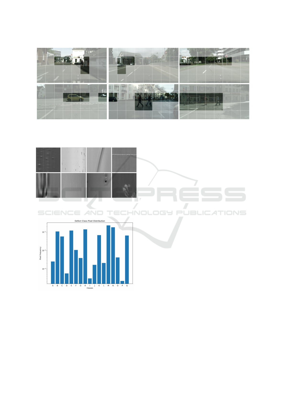
Figure 6: Patch based sampling, shown on a CityScapes example. By sampling patches instead of full images to label, the
limited labeling budget can be optimally spent. Also, during training, the model sees the full input image with only supervision
for pixels within labeled patches. This enables the model to see the global context of the image during training, in contrast to
training on small crops, which would reduce overall segmentation performance.
Figure 7: Some example images from the steel sheet seg-
mentation task. The dataset consists of 18 different defect
classes.
Figure 8: Class pixel distribution. The figure shows how
imbalanced the data is, making it difficult to train on. The
imbalance is caused by the different occurrence rate of de-
fects, as well as the varying sizes of the defects.
(e.g., small spots), and will focus on large uncertain
regions. Therefore, we averaged the uncertainty for
small patches of size 64×64, and selected the top 4
highest uncertain patches. Using this method, the un-
certainty score is able to also focus on very small re-
gions, which is crucial for this use case since a lot
of defects are very small. This way, we are able to
give equal weight to large as well as small uncertain
regions in the images, as can be seen in Figure 9.
For training the main task model, we follow the
setup described in (Neven and Goedem
´
e, 2021), by
using a standard U-Net architecture (Ronneberger
et al., 2015) trained with a weighted cross-entropy
loss. The results can be seen in Figure 10. We com-
pare our method against random sampling, and using
a DPP only. In each active learning step we sample
8000 images from the unlabeled data pool for a to-
tal of five steps. While only sampling images in the
representation space using a DPP already increases
the mIoU, including the main task model’s uncer-
tainty drastically increases the segmentation perfor-
mance by nearly 5 percent in the last step, which is
only 2 percent lower than the upper bound score when
labeling and training a model on all the images from
the unlabeled pool.
5 DISCUSSION
While we have shown the effectiveness of our method
and compared against recent active learning methods
on academic datasets, for an industrial use case, the
real bottleneck of active learning algorithms is the
computational overhead. Most of the time, the algo-
rithms require a separate model to be retrained each
active learning step (e.g., VAAL, Learning Loss, . . . ).
While they have shown to be effective, this is infea-
sible when dealing with a large dataset, which also
contain a lot of redundant data. Using our method,
we only need to train a separate model once, i.e., the
representation model, and only train the main task
VISAPP 2023 - 18th International Conference on Computer Vision Theory and Applications
102

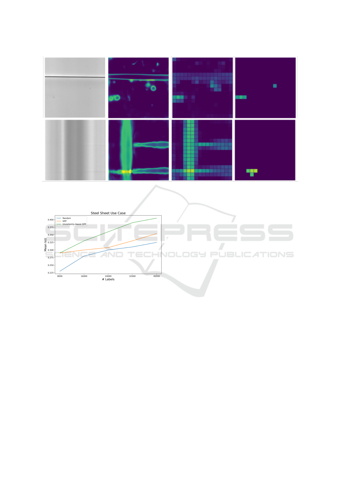
Figure 9: Example of main task model’s uncertainty for unlabeled images. Instead of averaging the uncertainty per image,
the uncertainty heatmap is divided into small patches. From these patches, the top 4 uncertain ones are averaged to compute
the final image uncertainty score. This ensures both small and large regions are equally weighed during sampling.
Figure 10: Active learning results for the industrial sheet
steel segmentation task. Results are averaged over 5 inde-
pendent runs.
model during the next active learning steps. The sam-
pling overhead between the steps is minimal, since we
only need to compute the uncertainty scores for each
unlabeled sample and adapt the pre-computed L ma-
trix. Compared to one epoch of training the main task
model, the DPP sampling time and compute can be
neglected. Therefore, this method of active learning
is especially suitable for large datasets and to drasti-
cally reduce computational overhead.
One other thing to remark is that, while train-
ing the representation model beforehand can be seen
as computational overhead, the weights of the model
can be a great initialization for the main task model.
Since the representation model learns abstract fea-
tures to distinguish different classes, these weights
would jumpstart the model and increase the score over
a random initialization. We did not include this in
our work because of the comparison with other ac-
tive learning methods, as training the main task model
needs to be separated from the active learning sam-
pling.
6 CONCLUSION
Active learning remains a key component when train-
ing computer vision models on industrial large-scale
datasets. In this work, we have introduced a new
active learning method that not only exceeds other
recent active learning methods, but also reduces
the overall computational overhead. By combining
model uncertainty with DPP sampling, we were able
to effectively sample diverse and informative data
points. First, we have shown the effectiveness of
our method on both academic classification and seg-
mentation benchmarks and extended our method to a
patch-based approach for semantic segmentation, in-
creasing the performance by further reducing data re-
dundancy within images. Last, we have shown the
robustness of our method on a challenging industrial
use case, which contained both a large class imbal-
ance and an abundance of redundant data.
Uncertainty-Aware DPP Sampling for Active Learning
103

ACKNOWLEDGEMENTS
This research received funding from the Flemish
Government (AI Research Program) and the VLAIO
project HBC.2021.0730. We thank Aperam for sup-
plying the steel surface defects dataset.
REFERENCES
Anari, N., Gharan, S. O., and Rezaei, A. (2016). Monte
carlo markov chain algorithms for sampling strongly
rayleigh distributions and determinantal point pro-
cesses.
Caramalau, R., Bhattarai, B., and Kim, T.-K. (2020). Se-
quential graph convolutional network for active learn-
ing.
Chen, L.-C., Papandreou, G., Kokkinos, I., Murphy, K., and
Yuille, A. L. (2016). Deeplab: Semantic image seg-
mentation with deep convolutional nets, atrous convo-
lution, and fully connected crfs.
Chen, T., Kornblith, S., Norouzi, M., and Hinton, G. (2020).
A simple framework for contrastive learning of visual
representations. arXiv preprint arXiv:2002.05709.
Cordts, M., Omran, M., Ramos, S., Rehfeld, T., Enzweiler,
M., Benenson, R., Franke, U., Roth, S., and Schiele,
B. (2016). The cityscapes dataset for semantic urban
scene understanding. In Proc. of the IEEE Conference
on Computer Vision and Pattern Recognition (CVPR).
Deng, J., Dong, W., Socher, R., Li, L.-J., Li, K., and Fei-
Fei, L. (2009). Imagenet: A large-scale hierarchical
image database. In 2009 IEEE Conference on Com-
puter Vision and Pattern Recognition, pages 248–255.
Dwibedi, D., Aytar, Y., Tompson, J., Sermanet, P., and Zis-
serman, A. (2021). With a little help from my friends:
Nearest-neighbor contrastive learning of visual repre-
sentations.
Fei-Fei, L., Fergus, R., and Perona, P. (2004). Learning gen-
erative visual models from few training examples: An
incremental bayesian approach tested on 101 object
categories. Computer Vision and Pattern Recognition
Workshop.
Freund, Y., Seung, H. S., Shamir, E., and Tishby, N. (1995).
Selective sampling using the query by committee al-
gorithm. In Machine Learning, pages 133–168.
Gautier, G., Polito, G., Bardenet, R., and Valko, M.
(2019). DPPy: DPP Sampling with Python. Jour-
nal of Machine Learning Research - Machine Learn-
ing Open Source Software (JMLR-MLOSS). Code
at http://github.com/guilgautier/DPPy/ Documenta-
tion at http://dppy.readthedocs.io/.
He, K., Fan, H., Wu, Y., Xie, S., and Girshick, R. (2019).
Momentum contrast for unsupervised visual represen-
tation learning.
He, K., Zhang, X., Ren, S., and Sun, J. (2016). Deep resid-
ual learning for image recognition. In 2016 IEEE Con-
ference on Computer Vision and Pattern Recognition
(CVPR), pages 770–778.
Joseph, K. J., Khan, S., Khan, F. S., and Balasubramanian,
V. N. (2021). Towards open world object detection.
Joshi, A. J., Porikli, F., and Papanikolopoulos, N. (2009).
Multi-class active learning for image classification. In
2009 IEEE Conference on Computer Vision and Pat-
tern Recognition, pages 2372–2379.
Kapoor, A., Grauman, K., Urtasun, R., and Darrell, T.
(2007). Active learning with gaussian processes for
object categorization. In 2007 IEEE 11th Interna-
tional Conference on Computer Vision, pages 1–8.
Krizhevsky, A. (2009). Learning multiple layers of features
from tiny images. Technical report.
Kulesza, A. (2012). Determinantal point processes for ma-
chine learning. Foundations and Trends® in Machine
Learning, 5(2-3):123–286.
Li, C., Jegelka, S., and Sra, S. (2016a). Fast sampling for
strongly rayleigh measures with application to deter-
minantal point processes.
Li, C., Sra, S., and Jegelka, S. (2016b). Fast mixing
markov chains for strongly rayleigh measures, dpps,
and constrained sampling. In Lee, D., Sugiyama,
M., Luxburg, U., Guyon, I., and Garnett, R., editors,
Advances in Neural Information Processing Systems,
volume 29. Curran Associates, Inc.
MacKay, D. J. C. (1992). Information-based objective func-
tions for active data selection. Neural Computation,
4(4):590–604.
McCallum, A. and Nigam, K. (1998). Employing em and
pool-based active learning for text classification. In
Proceedings of the Fifteenth International Conference
on Machine Learning, ICML ’98, page 350–358, San
Francisco, CA, USA. Morgan Kaufmann Publishers
Inc.
Neven, R. and Goedem
´
e, T. (2021). A multi-branch u-net
for steel surface defect type and severity segmenta-
tion. Metals, 11(6).
Ronneberger, O., Fischer, P., and Brox, T. (2015). U-net:
Convolutional networks for biomedical image seg-
mentation.
Sener, O. and Savarese, S. (2017). Active learning for con-
volutional neural networks: A core-set approach.
Sinha, S., Ebrahimi, S., and Darrell, T. (2019). Variational
adversarial active learning. In 2019 IEEE/CVF In-
ternational Conference on Computer Vision (ICCV),
pages 5971–5980.
Srinivas, A., Laskin, M., and Abbeel, P. (2020). Curl: Con-
trastive unsupervised representations for reinforce-
ment learning.
Tong, S. and Koller, D. (2002). Support vector machine
active learning with applications to text classification.
J. Mach. Learn. Res., 2:45–66.
Yoo, D. and Kweon, I. S. (2019). Learning loss for active
learning. In 2019 IEEE/CVF Conference on Com-
puter Vision and Pattern Recognition (CVPR), pages
93–102.
VISAPP 2023 - 18th International Conference on Computer Vision Theory and Applications
104