Improving Convergence for Quantum Variational Classiﬁers Using

Weight Re-Mapping

Michael K

olle, Alessandro Giovagnoli, Jonas Stein, Maximilian Balthasar Mansky, Julian Hager

and Claudia Linnhoff-Popien

Institute of Informatics, LMU Munich, Oettingenstraße 67, Munich, Germany

ﬁ

Keywords:

Variational Quantum Circuits, Variational Classiﬁer, Weight Re-Mapping.

Abstract:

In recent years, quantum machine learning has seen a substantial increase in the use of variational quantum

circuits (VQCs). VQCs are inspired by artiﬁcial neural networks, which achieve extraordinary performance

in a wide range of AI tasks as massively parameterized function approximators. VQCs have already demon-

strated promising results, for example, in generalization and the requirement for fewer parameters to train, by

utilizing the more robust algorithmic toolbox available in quantum computing. A VQCs’ trainable parameters

or weights are usually used as angles in rotational gates and current gradient-based training methods do not

account for that. We introduce weight re-mapping for VQCs, to unambiguously map the weights to an interval

of length 2π, drawing inspiration from traditional ML, where data rescaling, or normalization techniques have

demonstrated tremendous beneﬁts in many circumstances. We employ a set of ﬁve functions and evaluate

them on the Iris and Wine datasets using variational classiﬁers as an example. Our experiments show that

weight re-mapping can improve convergence in all tested settings. Additionally, we were able to demonstrate

that weight re-mapping increased test accuracy for the Wine dataset by 10% over using unmodiﬁed weights.

1 INTRODUCTION

Machine learning (ML) tasks are ubiquitous in a vast

number of domains, including central challenges of

humanity, such as drug discovery or climate change

forecasting. In particular, ML techniques allow to

tackle problems, for which computational solutions

were unimaginable before its rise. While many tasks

can be solved efﬁciently using machine learning tech-

niques, fundamental limitations are apparent in oth-

ers, e.g., the curse of dimensionality (Bellman, 1966).

Inspired by the success of classical ML and a promis-

ing prospect to circumvent some of its intrinsic lim-

itations, quantum machine learning (QML) has be-

come a central ﬁeld of research in the area of quantum

computing. Based on the laws of quantum mechan-

ics rather than classical mechanics, a richer algorith-

mic tool set can be used to solve some computational

problems faster on a quantum computer than classi-

cally possible. In some special cases, this new tech-

nology allows for exponential speedups for speciﬁc

problems, such as classiﬁcation and regression, i.e.,

by employing a quantum algorithm to solve systems

of linear equations (SLEs), whose runtime is logarith-

mic in the dimensions of the SLEs for sparse matrices

(Harrow et al., 2009). Aside from the application of

such provably efﬁcient basic linear algebra subrou-

tines, a central pillar of quantum computing, a new

ﬁeld in QML has recently been proposed: Variational

Quantum Computing (VQC). Using elementary con-

structs of quantum computing, a universal function

approximator can be constructed, much in the same

way as in artiﬁcial neural networks. In analogy to

logic gates, quantum gates are the fundamental algo-

rithmic building blocks. The mathematical operations

represented by quantum computing building blocks

are different from classical elements, as they describe

rotations and reﬂections, or concatenations of these in

a vector space. Rather than working in a general vec-

tor space, quantum computing acts on a Hilbert space

with exponentially more dimensions available with

increasing number of parameters. In essence, every

variational quantum circuit can be decomposed into

a set of parametrized single qubit rotations and un-

parmeterized reﬂections (Nielsen and Chuang, 2010).

While variational quantum computing has bene-

ﬁts such as fewer training parameters to optimize (Du

et al., 2020), many open problems remain in its prac-

tical application. The structure of a quantum circuit

is its own problem, where many different concatena-

Kölle, M., Giovagnoli, A., Stein, J., Mansky, M., Hager, J. and Linnhoff-Popien, C.

Improving Convergence for Quantum Variational Classiﬁers Using Weight Re-Mapping.

DOI: 10.5220/0011696300003393

In Proceedings of the 15th International Conference on Agents and Artiﬁcial Intelligence (ICAART 2023) - Volume 2, pages 251-258

ISBN: 978-989-758-623-1; ISSN: 2184-433X

 2023 by SCITEPRESS – Science and Technology Publications, Lda. Under CC license (CC BY-NC-ND 4.0)

251

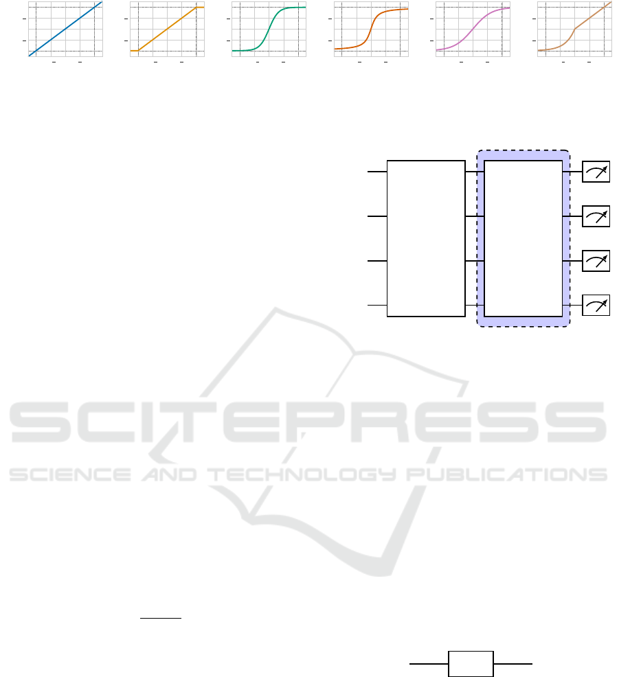
Figure 1: Overview of the Variational Quantum Circuit

Training Process with Weight Constraints.

tions of quantum gates are possible and lead to dif-

ferent training results. At the same time, the Hilbert

space is a closed space with possible values from

[0,2π]. It is still unclear how to best work with the

classically unusual domain restriction of the parame-

ters, set by the rotation operations. This problem is of

great relevance, as rotations, being periodic functions,

are not injective, and thus lead to ambiguous parame-

ter assignments and thus worse training performance.

Drawing inspiration from classical ML, where

data rescaling, or normalization techniques have

shown immense improvements in many cases (Singh

and Singh, 2019), we propose the introduction of re-

mapping training parameters in variational quantum

circuits as described in Figure 1. Concretely, we em-

ploy a set of well known ﬁxed functions to unambigu-

ously map the weights to an interval of length 2π and

test their performance. For evaluation purposes, we

use a classiﬁcation problem and a circuit architecture

suitable for the employed variational classiﬁer. Our

experimental data shows, that the proposed weight re-

mapping leads to faster convergence in all tested set-

tings compared to runs with unconstrained weights.

In some cases, the overall test accuracy can also be

improved. In this work, we ﬁrst describe the basics

of variational quantum circuits and related work. We

then explain the idea behind our approach and how

we setup up our experiments. Finally, we present and

discuss our results and end with a summary, limita-

tions and future work. All experiments and a PyTorch

implementation of the used weight re-mapping func-

tions can be found here

https://github.com/michaelkoelle/qw-map

2 VARIATIONAL QUANTUM

CIRCUITS

The most prominent function approximator used in

classical machine learning is the artiﬁcial neural net-

work: a combination of parameterized linear transfor-

mations and typically non-linear activation functions,

applied to neurons. The weights and biases used to

parameterize the linear transformations can be up-

dated using gradient based techniques like backprop-

agation, optimizing the approximation quality. Ac-

cording to Cybenko’s universal approximation theo-

rem, this model allows the approximation of arbitrary

functions with arbitrary precision.(Cybenko, 1989).

In a quantum circuit, information is stored in the

state of a qubit register

⟩

, i.e., normalized vectors

living in a Hilbert space H . In quantum mechanics,

a function mapping the initial state

⟩

onto the ﬁnal

state





is expressed by a unitary operator U that

maps the inputs onto the outputs as in





= U

⟩

In contrast to classical outputs, quantum outputs can

only by obtained via so called measurements, which

yield an eigenstate corresponding with an expected

value of







, where O is typically chosen to

be the spin Hamiltonian in the z-axis.

In order to build a quantum function approximator

in form of a VQC, one typically decomposes the arbi-

trary unitary operator U into a set of quantum gates.

Analogously to Cybenko’s theorem, in the quantum

case it can be proved that any unitary operator act-

ing on multiple qubits can always be expressed by

the combination of controlled-not (CNOT) and ro-

tational (ROT) gates, which represent reﬂections or

rotations of the vector into the Hilbert space respec-

tively (Nielsen and Chuang, 2010). While CNOTs are

parameter-free gates, each rotation is characterized by

the three angles around the axes of the Bloch sphere.

These rotation parameters are the weights of the quan-

tum variational circuit. We can thus say that the ﬁnal

state actually depends on the weights θ of the circuit,

and rewrite the output ﬁnal value as



(θ)



(θ)



(1)

Starting from this theoretical basis, a function approx-

imator can be obtained once a suitable circuit struc-

ture, also called ansatz, has been chosen. Once this

is done and an objective function has been chosen,

the rotation weights can be trained in a quantum-

classical pipeline, as shown in Figure 1, completely

analogously to what is done with a neural network.

Similar to a classical neural network, where the

gradient is calculated using backpropagation, we can

differentiate the circuit with respect to the parame-

ters θ in a similar way using the parameter shift rule

ICAART 2023 - 15th International Conference on Agents and Artiﬁcial Intelligence

252

(Schuld et al., 2019). It has to be noted however, that

this approach has linear time complexity in the num-

ber of parameters and every gradient calculation has

to be executed on a quantum computer. This is signif-

icantly worse than the constant time complexity re-

garding the number of parameters, needed in back-

propagation.

3 RELATED WORK

The task of embedding data from R

to SU(2

) has

received limited attention so far, with approaches fo-

cusing on global embeddings (Lloyd et al., 2020) or

local mappings. The former approach adds another

classical calculation overhead to the whole VQC con-

struction. It is also data speciﬁc and needs to be re-

trained for each dataset.

For local embeddings there are arguments for

rescaling the data classically to a ﬁxed interval as

[min(data),max(data)] → [0, 1] for each data dimen-

sion and then mapping that to rotations on a single

qubit axis (Stoudenmire and Schwab, 2016), multi-

qubit embedding (Mitarai et al., 2018) and random

linear maps (Wilson et al., 2019)(Benedetti et al.,

2019).

4 OUR APPROACH

In this section, we ﬁrst explain the idea and the pro-

cess behind weight re-mapping for variational quan-

tum circuits. Then we elaborate on the chosen exam-

ple implementation of a variational quantum classi-

ﬁer architecture and the datasets on which we evalu-

ate the approach. Note that, the approach is not lim-

ited to supervised learning tasks. Because weight re-

mapping can be applied to VQCs that act as function

approximators, it can be easily applied to other ma-

chine learning tasks such as unsupervised learning,

reinforcement learning, and so on. Finally, we detail

our training procedure and pre-tests that inﬂuenced

our architecture decisions.

4.1 Weight Re-Mapping

In a classical neural network the weights that charac-

terize the connections between the neurons are repre-

sented by a vector

⃗

θ ∈ R

. Once the neural network

has been evaluated and the back-propagation has been

performed, we obtain the gradient of the loss function

with respect to the parameters

⃗

θ, namely ∇

⃗

θ). The

weights are then updated as follows:

⃗

i−1

−α∇

⃗

i−1

⃗

i−1

) (2)

This update step relies on the fact that the space in

which we are moving to minimize the loss function

is R

, and thus every value of the real number line

can be assumed by the weights. The same is not true

in the case of quantum variational circuits, where, as

previously discussed, the parameters

⃗

θ represent ro-

tations around one of the three axes in the space of

the Bloch sphere. Since a rotation of angle θ around

a generic direction ˆv has a period of 2π, meaning

R( ˆv,θ) = R(⃗v,θ + 2π), it follows that for a parame-

ter θ that is close enough to the boundaries of the pe-

riod, updating the value according to (2) may result

in making the parameter end up in an adjacent period

and thus assume an unexpected value, possibly op-

posite to the desired direction. We can conclude that

the natural space where the parameters of a quantum

variational circuit should be taken is [φ, φ + 2π], with

φ ∈ R. To center the interval around the value 0 we

pick φ = −π. This way the parameters of a quantum

variational circuit are

⃗

θ ∈ [−π, π]

. In order to con-

strain the parameters in the interval [−π, π] we apply

a mapping function to the weights. A mapping func-

tion is any function of the type

ϕ : R → [a,b] (3)

that maps the real line to a compact interval. In

our case we are interested in a = −b = −π, so that

ϕ : R → [−π, π]. Introducing the mapping function

means that, whenever a forward pass in performed,

every rotation gate depending of a set of angles θ =

(θ

,θ

) will ﬁrst have its parameters remapped.

R(ϕ(θ))

We want to emphasize that because the parameters

⃗

will be constrained in the forward pass, they are al-

ways free to take values from the real line. This way

we can rewrite the basic update rule as follows:

⃗

i−1

−α∇

⃗

i−1

L(ϕ(

⃗

i−1

)) (4)

This shows that no mapping function is applied to

the weights during the update step, while it is dur-

ing the forward pass, represented by the loss function.

The mapping functions we decided to use in the ex-

periments are some of the most common functions

normally used to map the real numbers into a com-

pact interval, properly scaled in such a way that the

output interval is [−π,π]. First, we introduce the iden-

tity function, which serves as our baseline without a

weight constraint. This is equal to applying no map-

ping at all, as can be seen in Figure 2a.

Improving Convergence for Quantum Variational Classiﬁers Using Weight Re-Mapping

253

−π

−

Parameter value

−π

−

Mapped output

(a) No Re-

Mapping.

−π

−

Parameter value

−π

−

Mapped output

(b) Clamp.

−π

−

Parameter value

−π

−

Mapped output

−π

−

Parameter value

−π

−

Mapped output

(d) Arctan.

−π

−

Parameter value

−π

−

Mapped output

(e) Sigmoid.

−π

−

Parameter value

−π

−

Mapped output

(f) Elu.

Figure 2: Re-Mapping functions.

(θ) = θ (5)

Starting out with the ﬁrst mapping function in Figure

2b, we simply clamp all parameter values above π to

π and all values below −π to −π. Within the interval

[−π,π] the identity function is used.

(θ) =











−π if θ < −π

π if θ > π

θ otherwise

(6)

Next, we use the hyperbolic tangent function and ap-

ply a scaling of π. This creates a steeper mapping

around θ = 0 but has a smoother transition near −π

and π, as shown in Figure 2c

(θ) = πtanh(θ) (7)

After some initial tests, we wanted to explore the im-

pact of how fast the function approaches the bounds

−π and π. Therefore, we scaled the inverse tangent

function with factor 2 in both axes. Its graph is shown

in Figure 2d.

(θ) = 2arctan(2θ) (8)

Furthermore, we tested a modiﬁed sigmoid function,

which is not as steep as the previous two and ap-

proaches the bounds faster than ϕ

but slower than

. To archive the graph in Figure 2e, we needed to

scale the function with factor 2π and shift it by −π.

(θ) =

2π

1 + e

−θ

−π (9)

Lastly, we tested the Exponential Linear Unit or ELU

as a asymmetric function, expecting that it should not

work as good as the previously mentioned functions.

To make sure that the function at least converges to

the lower bound −π for θ < 0, we set its α parameter

to π. Its graph can be seen in Figure 2f.

(θ) =

(

π(e

−1) if θ < 0

θ otherwise

(10)

4.2 Variational Circuit Architecture

The variational quantum circuit used in the variational

classiﬁer consists of 3 parts (Figure 3).

⟩

Figure 3: Abstract variational quantum circuit used in this

work. Dashed blue area indicates repeated layers.

State Preparation

Initially, we start with the state preparation S

, where

the feature vector is embedded into the circuit. Here,

real values of the feature vector are mapped from the

Euclidean space to the Hilbert space. There are many

ways to embed data into a circuit and many differ-

ent state preparation methods. After a small scale

pre-test, we determined that the Angle Embedding

yielded the best results on both the Iris and Wine

dataset. Angle Embedding is a simple technique to

encode n real-valued features into n qubits. Each of

the qubits are initialized as

⟩

and then rotated by

some angle around either the x- or y-axis. The cho-

sen angle corresponds to the feature amplitude to be

encoded. Usually single axis rotational gates, are ap-

plied, as seen in the example

)

if we call x

∈ R the j-th feature to be embedded and

, with i ∈ {X,Y } the rotational gate around the i-

th axis, then the embedding is performed by simply

applying the gate represented below. Note that the

z-axis is left out: since the initial qubits are in the

⟩

state, which correspond in the Bloch sphere to vectors

along the z-axis, rotations around it naturally have no

effect and no information would be encoded.

ICAART 2023 - 15th International Conference on Agents and Artiﬁcial Intelligence

254

Variational Layers

The second part of the circuit L

, hereafter called lay-

ers, consists of repeated single qubit rotations and en-

tanglers (in Figure 3 everything contained within the

dashed blue area is repeated L times, where L is the

layer count). Speciﬁcally, we use a layer architec-

ture inspired by the circuit-centric classiﬁer design

(Schuld et al., 2020). All circuits presented in this

paper use three single qubit rotation gates and CNOT

gates as entanglers. Here, we show an example of the

ﬁrst layer L

of a three qubit variational classiﬁer.

RX(θ

)

RY (θ

) RZ(θ

)

RX(θ

)

RY (θ

) RZ(θ

)

RX(θ

)

RY (θ

) RZ(θ

)

In the circuit above θ

denotes a trainable parameter

where i represents the qubit index and j ∈{0, 1, 2}the

index of the single qubit rotation gate. For clarity, we

omitted the index l which denotes the current layer in

the circuit. In each layer, the target bit of the CNOT

gate is given by (i +l) mod n. For example, in the ﬁrst

layer l = 1 the control and target qubits are zero qubits

apart and are direct neighbors in a circular manner. In

the next layer l = 2, the control and target qubits are

one qubit apart. Continuing the example, the index of

the target qubit of qubit i = 0 is (0 + 2) mod 3 = 2.

Measurement

The last part of the circuit architecture is the measure-

ment. We measure the expectation value in the com-

putational basis (z) of the ﬁrst k qubits where k is the

number of classes to be determined. Then a bias is

added to each measured expectation value. The bi-

ases are also part of the parameters of the VQC and

are updated accordingly. Lastly, the softmax of the

measurement vector is computed in order to normal-

ize the probabilities.

4.3 Datasets

In this section, we present the datasets that were used

to assess the variational classiﬁer from section 4.2.

We chose two popular datasets that pose a simple su-

pervised learning classiﬁcation task.

4.3.1 Iris Dataset

The Iris dataset originates from an article by Fisher

(Fisher, 1936) in 1936. Since then it has been fre-

Table 1: Hyperparameters used for each dataset.

Parameter Iris Dataset Wine Dataset

Learning Rate 0.0201 0.0300

Weight Decay 0.0372 0.0007

Batch Size 9 18

Embedding Angle (X-Axis) Angle (Y-Axis)

Number of Layers 8 9

quently referenced in many publications to this day.

We are using a newer version of the dataset, where

two small errors were ﬁxed in comparison to the orig-

inal article. The dataset includes 3 classes with 50

instances each, where each class refers to one of the

following types of iris plants: Iris Setosa, Iris Versi-

colour, Iris Virginica. Each feature vector contains

sepal length (in cm), sepal width (in cm), petal length

(in cm) and petal width (in cm) respectively. The Iris

dataset is a particularly easy dataset to classify, espe-

cially when considered that the ﬁrst two classes are

linearly separable. The latter two classes are not lin-

early separable.

4.3.2 Wine Dataset

The Wine dataset was created in July 1991 as a result

of a chemical analysis of wines of three different cul-

tivars grown in the same region in Italy (Vandeginste,

1990). Originally, they investigated 30 constituents

but they were then lost to time and only a smaller

version of the dataset still remains. The remaining

dataset includes 3 classes which represent the differ-

ent cultivars, a total of 178 instances containing 13

features each: Alcohol, Malic acid, Ash, Alcalinity

of ash, Magnesium, Total phenols, Flavanoids, Non-

ﬂavanoid phenols, Proanthocyanins, Color intensity,

Hue, OD280/OD315 of diluted wines and Proline.

The dataset is not balanced and the instances are dis-

tributed among the classes as follows: class 1: 59,

class 2: 71, class 3: 48.

4.4 Training

We started the training of the variational classiﬁers

with a hyperparameter search using Bayesian opti-

mization. We trained approximately 300 runs per

dataset, optimizing the test accuracy. All runs in the

hyperparamter search were executed without weight

constraints. The hyperparameters of the best run for

each dataset can be found in Table 1. We then ran

20 runs for every mapping function on the Iris dataset

and 10 runs each on Wine dataset, each with the be-

fore mentioned hyperparameters. The initialization

of the weights is important when using weight con-

straints, since the functions deﬁned in Section 4.1

are centered around 0. Therefore, we initialized the

Improving Convergence for Quantum Variational Classiﬁers Using Weight Re-Mapping

255

Table 2: Test Accuracy of tested mapping functions with 95% conﬁdence interval.

Dataset w/o Re-Mapping Clamp Tanh Arctan Sigmoid ELU

Iris 0.953 ±0.024 0.953±0.024 0.953 ±0.024 0.957 ±0.023

0.957 ±0.023

0.957 ±0.023 0.950 ±0.025 0.943 ±0.026

Wine 0.617 ±0.071 0.622 ±0.071 0.706 ±0.067 0.667 ±0.069 0.717 ±0.066

0.717 ±0.066

0.717 ±0.066 0.694 ±0.067

Table 3: Accuracy (Validation) of tested mapping functions

during convergence.

Iris Dataset

Samples w/o Re-Mapping Clamp Tanh Arctan Sigmoid ELU

120 0.693 0.700 0.903 0.913

0.913

0.913 0.837 0.840

240 0.883 0.887 0.937

0.937

0.937 0.927 0.927 0.910

480 0.933 0.937

0.937

0.937 0.927 0.933 0.930 0.920

Wine Dataset

Samples w/o Re-Mapping Clamp Tanh Arctan Sigmoid ELU

568 0.372 0.372 0.533

0.533

0.533 0.522 0.489 0.511

994 0.511 0.517 0.639

0.639

0.639 0.539 0.583 0.533

1846 0.572 0.572 0.656

0.656

0.656 0.639 0.628 0.628

weights close to 0 in the range of [−0.01, 0.01]. For

the training we used Cross Entropy Loss and Adam

Optimizer.

5 EXPERIMENTS

In this section we present our conducted experiments

on the Iris and Wine datasets. To show the im-

pact of the re-mapping functions from Section 4.1,

we chose simple supervised learning tasks using a

quantum variational classiﬁer. However, in princi-

ple our approach can be used for any scenario that

relies on a variational quantum circuit, for example

Quantum Reinforcement Learning, QAOA, and more.

We trained the classiﬁer on two different datasets Iris

(Section 4.3.1) and Wine (Section 4.3.2). All train-

ing related details can be found in Section 4.4. We

ﬁrst investigated the convergence behavior with and

without the weight re-mapping. This is an important

topic, especially for quantum machine learning, since

the use of quantum hardware is much more expen-

sive than classical hardware at the time of writing.

In Figure 4 and Table 3 we show that faster conver-

gence can be achieved by using weight re-mapping

in all tested settings. With a faster convergence we

can potentially save on compute which results in less

power consumption and C0

emissions. We also in-

vestigated overall test accuracy in Table 2, where we

can see minor improvements for the Iris dataset and a

10% improvement for the Wine dataset, compared to

using no weight re-mapping.

5.1 Iris Dataset

In the following, we present the results of our ex-

periments on the Iris dataset. In a pre-test we

have found that Angle Embedding with rotations

around the x-axis works best for the classiﬁcation of

the Iris dataset, but also requires more qubits than

other embedding methods like Amplitude Embedding

ott

onen et al., 2005). It should be noted, that Angle

Embedding with rotations around the y-axis should, in

theory, perform similarly. Angle Embedding with ro-

tations around the z-axis does not work at all, since

the rotations are invariant to the expectation value of

the measurement w.r.t. z-axis. We then ran a quick

hyperparameter search on the architecture without a

re-mapping function, determining the hyperparame-

ters listed in Table 1. We wanted to see if we can fur-

ther improve the convergence of an architecture with

an already good set of hyperparameters, just by in-

troducing weight re-mapping. We trained the model

with and without weight re-mapping with 20 differ-

ent seeds on the dataset. The whole training curves

can be found in Figure 4 and the convergence behav-

ior can be seen in detail in Table 3, where we picked

three points during convergence and compared the ac-

curacies. We observe a increase of over 20% using the

Arctan re-mapping compared to using no re-mapping

after 120 samples. Similarly, after 240 samples the

model Tanh mapping has already converged and re-

sulted in over 5% higher accuracy. As the model with-

out re-mapping reaches convergence after 480 sam-

ples, we see practically no difference between the ap-

proaches. Theses differences can be attributable to

the re-mapping functions. In this particular case the

optimal weights are close to zero and especially Tanh

and Arctan are very steep in this area. One possibility

is that the re-mapping kept the values closer to this

area resulting in ﬁnding the weights faster. We also

investigated if the re-mapping process has any impact

on the overall test accuracy, where the results can be

found in Table 2. As expected, the test accuracy did

not decrease when using weight re-mapping for the

Iris dataset. It even reached a minimally higher test

accuracy which is due to more time for ﬁne-tuning

after the earlier convergence. In this setting, Arctan

is our overall preferred choice because of its fast con-

vergence and second best test accuracy.

5.2 Wine Dataset

The results of our experiments on the Wine dataset are

presented below. In a preliminary test, we discovered

that, in contrast to the Iris dataset, Angle Embedding

ICAART 2023 - 15th International Conference on Agents and Artiﬁcial Intelligence

256

0 2 4 6 8 10

0.6

0.8

1.0

Accuracy (Validation)

Iris Dataset

0 10 20 30 40 50

0.4

0.6

0.8

Wine Dataset

0 2 4 6 8 10

Epoch

0.8

0.9

1.0

Loss (Validation)

0 10 20 30 40 50

Epoch

0.9

1.0

1.1

w/o Re-Mapping

Clamp

Tanh

Arctan

Sigmoid

ELU

Figure 4: Validation curves for datasets Iris and Wine. In each epoch the algorithm processes 80% of the total samples of each

dataset for training. This accounts to 120 samples for the Iris dataset and 142 samples for the Wine dataset.

with rotations around the y-axis works best. In theory,

Angle Embedding with rotations around the x-axis

should perform similarly, since we are measuring the

expectation value w.r.t. z-axis and rotations around

the z-axis do not work at all, since the rotations are

invariant to the expectation value of the measurement.

Like the architecture used for the Iris dataset, Angle

Embedding outperformed more efﬁcient embedding

methods like Amplitude Embedding (M

ott

onen et al.,

2005). The architecture without a re-mapping func-

tion was then also subjected to a small scale hyperpa-

rameter search, yielding the hyperparameters listed in

Table 1. We were interested in determining whether

adding weight re-mapping may further enhance the

convergence of an architecture with a good set of hy-

perparameters. On the dataset, we trained the model

both with and without weight re-mapping using 20

seeds. The entire training curves are shown in Figure

4, and Table 3 shows the convergence behavior in de-

tail, comparing the accuracies at three points during

convergence. From the results, we can see that Tanh

is outperforming all other tested settings during con-

vergence and models with weights re-mapping gener-

ally converging faster than the baseline. At 568 sam-

ples Tanh has a 15% higher accuracy compared to the

model without weight re-mapping. After 994 sam-

ples Tanh is almost fully converged, while the base-

line only converges long after 1846 samples. We be-

lieve that the cause of this effect is the same as that

mentioned in the section above. These differences

are brought on by the re-mapping operation. In this

case, the ideal weights are almost zero, and Tanh is

very steep in this region, mapping the values close

to zero and enabling a more detailed search in this re-

gion, ultimately resulting in a faster convergence. Ad-

ditionally, Table 2 shows that the weight re-mapping

not only leads to a faster convergence but also, in this

case, a 10% improvement in test accuracy, closely fol-

lowed by Tanh. Tanh is our ﬁrst preference in this sit-

uation because of its quick convergence and second-

best test accuracy.

6 CONCLUSION

In this work, we introduced weight re-mapping for

variational quantum circuits, a novel method for

accelerating convergence using quantum variational

classiﬁers as an example. In order to test our clas-

siﬁer on two datasets — Iris and Wine — we ﬁrst

conducted an initial hyperparameter search to identify

a good set of parameters without re-mapping. After

that, we introduced our weight re-mapping approach

for evaluation. Our experiments show that weight re-

mapping can improve convergence in all tested set-

tings. Faster convergence may allow us to lower the

amount of compute we need, which will reduce power

consumption and C0

emissions. This is crucial, es-

pecially for quantum machine learning, where access

to quantum hardware is quite expensive. Furthermore,

for the Wine dataset, we were able to demonstrate that

using weight re-mapping improved test accuracy by

10% compared to using unmodiﬁed weights. For both

settings, we would recommend a re-mapping function

that is steep around the initialization point, such as

Arctan and Tanh.

There are additional opportunities based on our

ﬁndings. This includes testing other datasets, with

more features or more complex classiﬁcation prob-

lems. We also see opportunities to develop special-

ized optimizers that take into account the unique char-

Improving Convergence for Quantum Variational Classiﬁers Using Weight Re-Mapping

257

acteristics of parameters in quantum circuits. Finally,

more research is required to determine the impact of

weight re-mapping on other tasks and ﬁelds, such as

Quantum Reinforcement Learning.

REFERENCES

Bellman, R. (1966). Dynamic programming. Science,

153(3731):34–37.

Benedetti, M., Lloyd, E., Sack, S., and Fiorentini, M.

(2019). Parameterized quantum circuits as machine

learning models. Quantum Science and Technology,

4(4):043001.

Cybenko, G. (1989). Approximation by superpositions of

a sigmoidal function. Math. Control. Signals Syst.,

2(4):303–314.

Du, Y., Hsieh, M.-H., Liu, T., and Tao, D. (2020). Expres-

sive power of parametrized quantum circuits. Physical

Review Research, 2(3).

Fisher, R. A. (1936). The use of multiple measurements in

taxonomic problems. Annals of eugenics, 7(2):179–

188.

Harrow, A. W., Hassidim, A., and Lloyd, S. (2009). Quan-

tum algorithm for linear systems of equations. Physi-

cal Review Letters, 103(15).

Lloyd, S., Schuld, M., Ijaz, A., Izaac, J., and Killoran, N.

(2020). Quantum embeddings for machine learning.

arXiv:2001.03622 [quant-ph].

Mitarai, K., Negoro, M., Kitagawa, M., and Fujii, K.

(2018). Quantum circuit learning. Phys. Rev. A,

98:032309.

ott

onen, M., Vartiainen, J. J., Bergholm, V., and Salo-

maa, M. M. (2005). Transformation of quantum states

using uniformly controlled rotations. Quantum Info.

Comput., 5(6):467–473.

Nielsen, M. A. and Chuang, I. L. (2010). Quantum Com-

putation and Quantum Information: 10th Anniversary

Edition. Cambridge University Press.

Schuld, M., Bergholm, V., Gogolin, C., Izaac, J., and Kil-

loran, N. (2019). Evaluating analytic gradients on

quantum hardware. Physical Review A, 99(3):032331.

arXiv:1811.11184 [quant-ph].

Schuld, M., Bocharov, A., Svore, K. M., and Wiebe, N.

(2020). Circuit-centric quantum classiﬁers. Physical

Review A, 101(3).

Singh, D. and Singh, B. (2019). Investigating the impact

of data normalization on classiﬁcation performance.

Applied Soft Computing, page 105524.

Stoudenmire, E. and Schwab, D. J. (2016). Super-

vised Learning with Tensor Networks. In Lee, D.,

Sugiyama, M., Luxburg, U., Guyon, I., and Garnett,

R., editors, Advances in Neural Information Process-

ing Systems, volume 29. Curran Associates, Inc.

Vandeginste, B. (1990). Parvus: An extendable package of

programs for data exploration, classiﬁcation and cor-

relation, m. forina, r. leardi, c. armanino and s. lanteri,

elsevier, amsterdam, 1988, price: Us $645 isbn 0-444-

43012-1. Journal of Chemometrics, 4(2):191–193.

Wilson, C. M., Otterbach, J. S., Tezak, N., Smith,

R. S., Polloreno, A. M., Karalekas, P. J., Heidel, S.,

Alam, M. S., Crooks, G. E., and da Silva, M. P.

(2019). Quantum Kitchen Sinks: An algorithm for

machine learning on near-term quantum computers.

arXiv:1806.08321 [quant-ph].

ICAART 2023 - 15th International Conference on Agents and Artiﬁcial Intelligence

258