Trading Strategy Validation Using Forwardtesting with Deep Neural

Networks

Ivan Letteri

, Giuseppe Della Penna

, Giovanni De Gasperis

and Abeer Dyoub

Department of Information Engineering, Computer Science and Mathematics,

University of L’Aquila, via Vetoio, Coppito, L’Aquila, Italy

Keywords:

Neural Networks, Machine Learning, Stock Trading, Stock Market Prediction, Quantitative Finance,

Algorithmic Trading, Technical Analysis.

Abstract:

Traders commonly test their trading strategies by applying them on the historical market data (backtesting),

and then reuse on their (future) trades the strategy that achieved the maximum proﬁt on such past data. In this

paper we propose a novel technique, that we shall call forwardtesting, that determines the strategy to apply by

testing it on the possible future predicted by a deep neural network that has been designed to perform stock

price forecasts and trained with the market historical data. Our results conﬁrm that neural networks outperform

classical statistical techniques when performing such forecasts, and their predictions allow to select a trading

strategy that, when applied to the real future, results equally or more proﬁtable than the strategy that would be

selected through the traditional backtesting.

1 INTRODUCTION

Stock market forecasting is a crucial task for investors

and an interesting research area in the ﬁnancial do-

main, since a good prediction can achieve high re-

turns. However, there are considerable challenges in

accurately predicting stock market trends due to their

chaotic and non-linear nature.

Traditional statistical models, which have been

extensively applied to market trend prediction so far,

can easily handle only linear or stationary data series

and manage limited amounts of information. On the

other hand, machine learning methods are being cur-

rently employed in a variety of complex tasks, for ex-

ample to classify cyber attacks (e.g., (Letteri et al.,

2018; Marín et al., 2021)), predict network trafﬁc

anomalies (e.g., (Letteri et al., 2019b; Sokolov et al.,

2019)), predict the course of a disease or, in the ﬁ-

nancial ﬁeld, for stock market forecasting (Kumbure

et al., 2022) or foreign exchange trading (Hryshko

and Downs, 2004). Between such methods, artiﬁcial

neural networks (ANN) and, in particular, deep neu-

ral networks (DNN) proved most suitable for dealing

https://orcid.org/0000-0002-3843-386X

https://orcid.org/0000-0003-2327-9393

https://orcid.org/0000-0001-9521-4711

https://orcid.org/0000-0003-0329-2419

with non-linear problems with multiple inﬂuencing

factors. Indeed, they are often used for image recog-

nition and natural language processing (e.g., (Soniya

et al., 2015), but are being applied also to the ﬁnan-

cial market (e.g., (Lu and Ohta, 2002; Lee and Chiu,

2002; Day and Lee, 2016)). Actually, the experiments

reported in this paper conﬁrm that DNNs achieve the

best overall accuracy in the price forecast task un-

der consideration, even if they require more time to

be tuned, if compared with state-of-the-art statistical

models such as ARIMA and Prophet.

Typically, traders test their (algorithmic trading)

strategies, i.e., the technical indicators to consider and

how to react to their values, on the historical market

data (the so called backtesting), and then apply to the

future trades the strategy that achieved the maximum

proﬁt on such past data. In this paper we propose a

framework that uses ﬁnancial market historical data

to train a set of DNNs in order to forecast the future

stock prices. Such predictions are then exploited in

a novel way, that we shall call forwardtesting, to de-

termine the most proﬁtable technical indicator(s) to

be used as the basis of a trading strategy that is then

executed by a robot advisor. In particular, with for-

wardtesting, the best strategy is devised by looking

at the proﬁts earned by applying the candidate strate-

gies directly to the possible future predicted by the

DNNs. In this way, we leverage on the capabilities

Letteri, I., Della Penna, G., De Gasperis, G. and Dyoub, A.

Trading Strategy Validation Using Forwardtesting with Deep Neural Networks.

DOI: 10.5220/0011715300003494

In Proceedings of the 5th International Conference on Finance, Economics, Management and IT Business (FEMIB 2023), pages 15-25

ISBN: 978-989-758-646-0; ISSN: 2184-5891

 2023 by SCITEPRESS – Science and Technology Publications, Lda. Under CC license (CC BY-NC-ND 4.0)

of the DNNs to learn from the past trends and char-

acteristics that would be difﬁcult or even impossible

to capture using the simple indicator-based analyses

performed by the classical approach. In such sense,

forwardtesting is able to better exploit the available

historical data and allow a ﬁner strategy deﬁnition.

To verify our approach, we test it on two shares is-

sued by companies operating in completely different

sectors. Such shares have only a common characteris-

tic in the period of time in which we have carried out

our analysis: a medium volatility (see, e.g., (Mehra,

1998)), i.e., price ﬂuctuations that are not excessively

large or small (as the ones, e.g., of a tech company

stock or a large blue-chip company stock, respec-

tively). The experiments show that our forwardtesting

technique allows the trader to choose a strategy that is

more or equally proﬁtable than the one that would be

selected through the traditional backtesting, if applied

on the same historical data. Therefore, forwardtesting

appears a promising strategy selection criterion.

The paper is organised as follows. In Section 2 we

introduce the dataset used to validate our approach,

and show several metrics that conﬁrm its generality

and adequacy to this task. Then, in Section 3 we show

the performances of two well-known statistical pre-

dictors on such dataset. In Section 4 the same fore-

cast task is accomplished using a speciﬁcally-tailored

deep neural network, showing that it achieves better

prediction accuracy and is therefore more suitable to

be used as the basis of our trading strategy selection

technique, which is introduced in Section 5 and vali-

dated by comparing its proﬁts with the ones deriving

from the strategy devised through the common back-

testing approach. Finally, Section 6 reports our con-

clusions and outlines our future research on this ﬁeld.

2 THE DATASET

To validate the methodology proposed in this pa-

per, we use the stock price data of the shares issued

by Abercrombie & Fitch Co. (ANF) and EOG Re-

sources, Inc. (EOG), both listed on the New York

Stock Exchange (NYSE).

ANF was founded at the end of September 1996,

and from April to October 2011 it was several times

close to the all-time high, always encountering resis-

tance. On November 23, 2021 the company CEO

announced net sales of $905 million, up 10% as

compared to the previous year and up 5% as com-

pared to the 2019 third quarter net sales (source:

(Global Newswire, 2021)). Figure 1 shows the ANF

stock price trends starting from October 30th, 2011 to

November 30th, 2021.

On the other hand, the EOG stock, with a market

value of $55.21 billion and 84.08% institutional own-

ership, has gained 9.39% so far (source: (Investope-

dia, 2019)). The company is expected to post quar-

terly earnings of $3.24 per share in its next report.

Figure 2 shows the EOG stock price trends in the

same time interval used for ANF.

ANF and EOG are certainly assets with a some-

times controversial trend and consequently well prof-

itable if rightly exploited, especially in 2020/2021,

due to the global pandemic. However, in the analysed

period, ANF and EOG do not appear the classic al-

ways proﬁtable stocks (e.g. Tesla, Apple, Microsoft,

or Bitcoin) to which trivially apply a passive buy and

hold strategy (Investopedia, 2020).

The dataset used in this paper consists of the

time series of OHLC prices for the above mentioned

stocks, over the time period from October 30, 2011 to

November 30, 2021, for a total of 2537 open market

days. OHLC prices are the opening, highest, lowest

and closing prices of an asset, and are commonly used

to analyse the assets price history when performing

the so called technical analysis (TA) to explore trad-

ing opportunities. The time series of price observa-

tions can be downloaded from Yahoo Finance (e.g.,

(Yahoo Finance, 2020)). The authors github reposi-

tory (temporarily hidden for double-blind evaluation)

also contains a copy of such data preprocessed and

split into train and test sets to be used in a deep neural

network.

2.1 Outliers Detection

Even if we already know that the assets in our dataset

have a medium volatility, we performed further anal-

yses in order to ﬁnd possible trend anomalies. In par-

ticular, we observed the monthly trend of the closing

price and the ﬁnancial return for both the assets, look-

ing for anomalies through the TSOD library (DHI So-

lution Software, 2022).

The results, illustrated in Figure 3, show that, for

what concerns the closing prices, there are only few

outliers in both trends. In particular, the algorithm

identiﬁed temporary bursts and correctly marked the

most pointed spikes (quick price changes) as anoma-

lies.

2.2 Synchrony Between Time Series

We included in our dataset two different shares in

order to prove that the proposed approach is gen-

eral enough to adapt to a variety of different shares

with medium volatility. However, for this to be true,

we also have to prove that the corresponding price

FEMIB 2023 - 5th International Conference on Finance, Economics, Management and IT Business

Figure 1: ANF average trend from October 30th, 2011 to November 30th, 2021.

Figure 2: EOG average trend from October 30th, 2011 to November 30th, 2021.

time series are completely uncorrelated, i.e., ANF and

EOG does not inﬂuence each other. Therefore, after

scaling the values with a minMax normalisation, we

evaluated the synchrony between the two ﬁnancial as-

sets using the Pearson coefﬁcient and the Dynamic

Time Warping.

The Pearson coefﬁcient measures the linear rela-

tion between two continuous signals, and is deﬁned as

r =

∑

−¯x)(y

−¯y)

√

∑

−¯x)

√

∑

−¯y)

, where x

and y

are, in our

case, the closing prices of the ANF and EOG stocks.

Coefﬁcients −1 and 1 indicate a perfect negative and

positive correlation, respectively, whereas 0 stands for

no correlation. It is worth noting that the Pearson co-

efﬁcient is highly sensible to outliers, which can al-

ter the correlation estimation, and requires the com-

pared time series to contain homoscedastic data, hav-

ing an homogeneous variance in the observation in-

terval. However, as shown in Section 2.1, both the

considered time series do not contain many outliers

and can be considered homoscedastic thanks to the

medium volatility of the corresponding stock prices.

The overall Pearson coefﬁcient between ANF and

EOG is 0.28, which conﬁrms that the two stocks are

almost completely uncorrelated. However, this is a

measure of the global synchrony in the overall period.

Therefore, for sake of completeness, we also calcu-

lated the local synchrony in small portions of the over-

all period by repeating the process along a moving

window of 120 samples. Figure 4 plots such moment-

by-moment synchrony curve, which conﬁrms our de-

ductions.

On the other hand, the Dynamic Time Warp-

ing (DTW) algorithm outperforms the Pearson cor-

relation in detecting atypical functional dependencies

(Linke et al., 2020) between time series, even if they

have a different number of samples. It calculates the

optimal match between the two series by minimising

the Euclidean distance between pairs of samples at the

same time.

Applied on our data, the DTW algorithm deter-

mined that, for the optimal match between the closing

prices of the ANF and EOG assets, the minimum path

cost is d = 209.95, and such a large distance between

the two stocks supports our hypothesis of a complete

absence of inﬂuence between them.

2.3 Stationarity Test

A time series is considered stationary when statis-

tical properties such as mean, variance, and covari-

ance are constant over time. For making predictions,

especially with statistical methods, stationarity is a

preferred characteristic. Otherwise, more complex

prediction algorithms, such as neural networks, are

preferable.

To test whether the time series in our dataset are

stationary, we use the stationary unit root as a sta-

tistical test. In particular, we used the Augmented

Dickey Fuller (ADF) test by analysing the test statis-

tic (TS), p-value, and critical value at 1%, 5%, and

10% conﬁdence intervals, with a number of lags au-

tomatically selected through the Akaike Information

Criterion (AIC) (Akaike, 1974).

Table 1 shows the stationarity test results. The p-

value results above the threshold (such as 5% or 1%)

and this conﬁrms that the time series are not station-

ary.

Trading Strategy Validation Using Forwardtesting with Deep Neural Networks

Figure 3: Anomaly detection in closing prices for ANF (left) and EOG (right).

Figure 4: Pearson correlation between ANF and EOG from October 30th, 2011 to November 20th, 2021.

3 FORECASTING WITH

STATISTICAL METHODS

The trading strategy presented in Section 5 is based

on the possible future predicted from the stock his-

torical price data. In order to choose the best fore-

cast methodology suitable for this task, we ﬁrst tested

the performances of two well-known statistical time

series forecasting methods, i.e., the ARIMA autore-

gressive model and the Prophet procedure, applied to

our dataset.

3.1 ARIMA Model

The well-known linear regression (LR) model has

various forms, such as the autoregressive (AR) model,

the moving average (MA) model, the autoregres-

sive moving average (ARMA) model, and its evo-

lution, the autoregressive integrated moving average

(ARIMA) model (Marquez, 1995).

In general, an ARIMA model needs three param-

eters to run: the number of autoregressive terms p,

the number of nonseasonal differences needed for sta-

tionarity d, and the number of lagged forecast er-

rors in the prediction equation q (see, e.g., (Marquez,

1995) for more information on the meaning of such

parameters). In our experiments, we used the Auto-

ARIMA algorithm implemented in the pmdarima li-

brary (Smith, 2022), which automatically discovers

the optimal parameters by performing differentiation

tests (i.e., Kwiatkowski-Phillips-Schmidt-Shin, Aug-

mented Dickey-Fuller, or Phillips-Perron) to deter-

mine d, and then trying various sets of p and q to min-

imise the selected criterion that is, in our case, AIC,

since it provides a good trade-off between the model

ﬁtting and the evaluation simplicity (Stoica and Se-

len, 2004) and also deals with the risk of overﬁtting

and underﬁtting. The lower is the AIC value, the bet-

ter is the result.

Table 2 shows that the best ARIMA model for

ANF has p = 0, d = 1, and q = 1, also known as

simple exponential smoothing model. On the other

hand, EOG has p = 0, d = 1, and q = 0, also known

as random walk model (Danyliv et al., 2019), where

t+1

= y

+ ε

, and ε

are a sequence of centred, un-

correlated random variables.

Figure 5 shows the predictions on the closing

prices made with such auto-selected optimal ARIMA

models for n = 30 days following the training times-

pan, which corresponds to the 2507 days of market

from October 30th, 2011 to October 16th, 2021. Note

that, in the following, for the sake of brevity we will

omit the graphs and values of low, high, and open

prices, since the forecast errors are always very simi-

lar between the four OLHC components.

Such forecasts are then compared with the actual

closing prices of the considered 30 days, in order to

evaluate the following error metrics:

• Mean Square Error(MSE): the average of the

squared difference between the correct and pre-

dicted values (called prediction error or residual);

• Root Mean Square Error (RMSE): the square root

of MSE, measuring the standard deviation of the

errors;

• Mean Absolute Error (MAE): the average of the

absolute differences between the correct and pre-

dicted values;

• Mean Absolute Percentage Error (MAPE): the av-

erage of the absolute errors (as in MAE) nor-

FEMIB 2023 - 5th International Conference on Finance, Economics, Management and IT Business

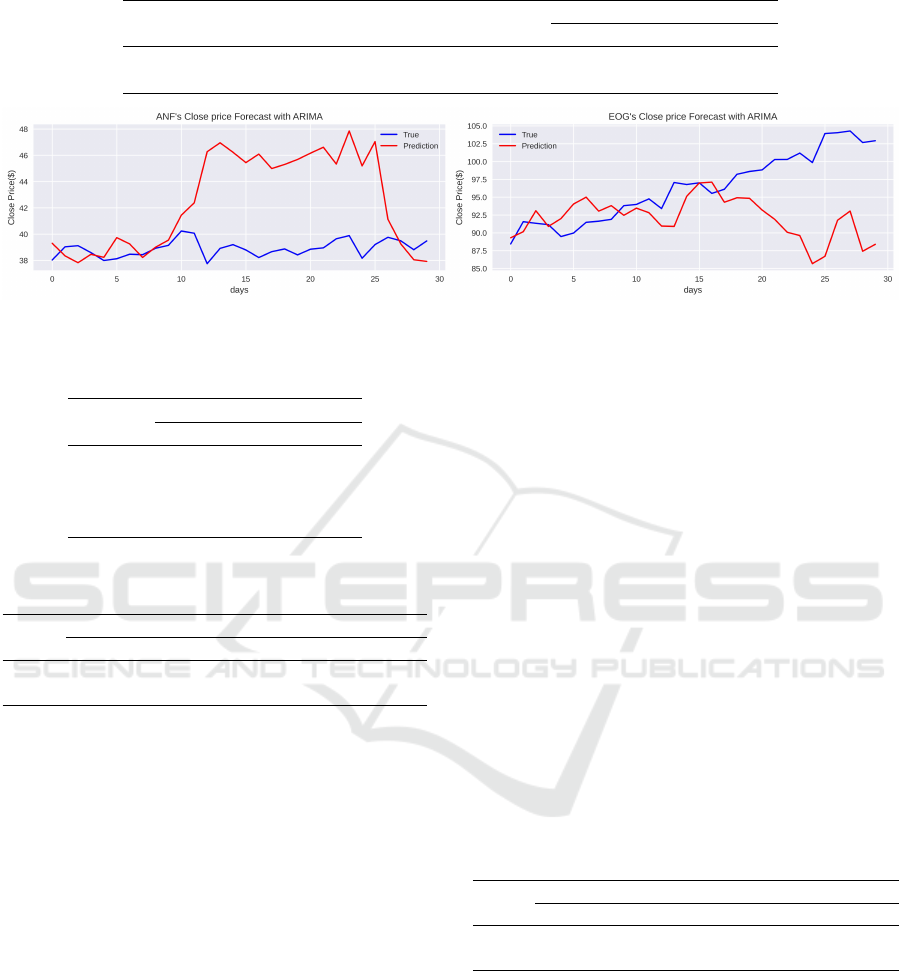
Table 1: ADF stationarity test with AIC optimization.

Critical Value

TS p-value Lags Observations 1% 5% 10%

ANF -2.302 0.171 5 2529 -3.432 -2.863 -2.567

EOG -2.422 0.135 5 2529 -3.433 -2.862 -2.567

Figure 5: Detail of ARIMA forecast for the last 30 days of the ANF (left) and EOG (right) stock closing prices.

Table 2: Step-wise search of the ARIMA (p,d,q) model that

minimises AIC for ANF and EOG.

AIC

( p,d,q ) ANF EOG

( 0,1,0 ) 8323.575 10369.768

( 1,1,0 ) 7652.108 10371.676

( 0,1,1 ) 7294.347 10371.541

( 1,1,1 ) 8317.976 10373.750

Table 3: Error metrics of ARIMA on ANF and EOG stock

price prediction.

ARIMA

MSE RMSE MAE MAPE EVS

ANF 25.49 5.05 3.86 0.09 -0.02

EOG 56.23 7.50 5.42 0.06 -3.94

malised w.r.t. to the correct values;

• Explained Variance Regression Score (EVS):

measure of the error dispersion (scores close to

1 are best).

Table 3 reports very high error metrics. It is worth

noting that the model performs a bit better with the

EOG stock, but not enough to be considered a suitable

tool for forecasting.

3.2 Prophet Model

Looking for a statistical method to improve the

ARIMA’s results, we turned to Facebook Prophet (see

(Žuni

c et al., 2020)). Prophet is ’a procedure for fore-

casting time series based on an additive model where

non-linear trends are ﬁt with yearly, weekly, and daily

seasonality, plus holiday effects. It works best with

time series that have strong seasonal effects and sev-

eral seasons of historical data. Prophet is robust to

missing data and shifts in the trend, and typically han-

dles outliers well’ (Facebook Open Source, 2022).

More technically, Prophet is an additive regressive

model which uses a time series with three main com-

ponents: trend, seasonality, and holidays, combined

in the equation y(t) = g(t) + s(t) + h(t) + ε(t), where

g(t) is the trend function which models non-periodic

changes in the value of the time series, s(t) represents

the seasonality, i.e., periodic changes (e.g., the num-

ber of trades might also depend on the month/year),

h(t) represents the effects of holidays, which have a

clear impact on most business time series, and ε(t) is

the error term, following a normal distribution. In our

experiments, we used Prophet ’out of the box’, leav-

ing all the default parameter selections.

Figure 6 shows, for the ANF and EOG closing

prices, the historical data as dots (where the right-

most red ones are the future to per predicted), and

the Prophet forecasts as a blue line. It is clear that

the model performs well in the ﬁrst years but, when

volatility increases (approximately in year 2020), the

forecasts start to be clearly worse.

Table 4: Error metrics of Prophet on ANF and EOG stock

price prediction.

Prophet

MSE RMSE MAE MAPE EVS

ANF 53.04 7.28 6.71 0.16 0.31

EOG 713.61 26.71 26.54 0.30 -0.03

Table 4 reports the corresponding error metrics

calculated in the same time frame used for the

ARIMA experiments. Clearly, the performances are

unacceptable also in this case.

3.3 Non Parametric Statistical Methods

For completeness in the statistical analysis, we also

evaluated non-parametric time series in statistical

models which do not rely on the assumption of a spe-

Trading Strategy Validation Using Forwardtesting with Deep Neural Networks

Figure 6: Detail of Prophet forecast for the ANF (left) and EOG (right) stock closing prices.

ciﬁc underlying distribution of the data (Mondal et al.,

2019). In the context of asset price forecasting, the

most commonly used method is the Spearman’s Rank

Correlation (SRC). SRC can be used to determine the

relationship between the asset’s past prices and its fu-

ture prices as follows: (i) Ranking historical prices in

ascending order, assigning the lowest price the rank

1 and the highest price the rank N, where N is the

number of prices in the time series. (ii) Calculate the

Spearman’s rank correlation:

ρ =

∑

i=1

−

R)(S

−

∑

i=1

−

∑

i=1

−

where R

and S

are the ranks of the i

observations,

R and

S are the mean ranks, and n is the number

of observations. (iii) Make the prediction: If there

is a strong positive correlation between the historical

price ranks and the forecast price ranks, it is possi-

ble to conclude that future asset prices will tend to

increase as historical prices increase.

Table 5: Error metrics of Spearman’s Rank Correlation on

ANF and EOG stock price prediction.

Spearman’s Rank Correlation

MSE RMSE MAE MAPE EVS

ANF 202.02 14.21 12.20 0.28 -3.15

EOG 10.84 3.29 2.72 0.03 -0.25

Table 5 reports the results about the errors,

and Figure 7 shows the limitations in forecasting

stock market prices of this non-parametric statistical

method. These are due to the complexity to cope

when dealing with large amounts of data. Another

problem is that are prone to overﬁtting that can result

in models that ﬁt the training data well but perform

poorly on new, unseen data.

4 FORECASTING WITH DEEP

LEARNING METHODS

Compared with conventional artiﬁcial neural net-

works, deep neural networks are characterised by a

higher number of neurons and hidden layers each of

which, in principle, gives the network a greater abil-

ity to extract high-level features. This makes DNNs

very efﬁcient in solving nonlinear problems: in partic-

ular, when it comes to time series forecasting, DNNs

can ﬁll the gap left open by traditional statistical tech-

niques such as the ones presented in Section 3, which

often assume that the series are generated by linear

processes and consequently may be inappropriate for

most real-world problems that are overwhelmingly

non-linear. Indeed, works like (Yao et al., 1999) and

(Hansen et al., 1999) (focusing on time series predic-

tion) show that neural network models often outper-

form conventional ARIMA models, and in particu-

lar (Hansen et al., 1999) also shows that neural net-

works outperform ARIMA in predicting the direction

of stock prices movements, since they are able to de-

tect hidden patterns in the time series.

In this section, we maintain the same forecasting

objective of Section 3, i.e., n = 30 days following the

training date. However, while the Auto-ARIMA de-

tected that the optimal conﬁguration for such an algo-

rithm was to generate a forecast based on the previ-

ous value only (see Section 3.1), here we empirically

found that the neural network performs better if its in-

put layer is fed with the t = 5 previous values, i.e., the

prices of the previous market week. In other words, to

forecast the price of a day s, the input neurons will be

presented to the prices of days s −1, . . . , s −5, respec-

tively. The network then outputs its price prediction

via a single neuron in the output layer.

When building a neural network for applications

like ﬁnancial forecasting, one must ﬁnd a compromise

between generalisation and convergence. For exam-

ple, hidden layers must not have too many nodes,

since they may lead the DNNs to learn the training

data without performing any generalisation. There-

fore, to ﬁnd the geometry (number and size of hid-

den layers) which minimises the error on all the net-

works, we developed a python module that generates

different network geometries in combination with the

sklearn GridSearchCV algorithm (scikit-learn, 2022)

, which in turn tries to ﬁnd the optimal combination

of the hyper parameters (epochs, batch size, learning

rate, optimiser employed) for each speciﬁc network.

The resulting optimal geometry has two hidden

layers composed by 10 ∗t and 5 ∗t neurons, respec-

tively, as in (Letteri et al., 2018) and (Letteri et al.,

2019b). In addition, to help reducing overﬁtting, we

FEMIB 2023 - 5th International Conference on Finance, Economics, Management and IT Business

Figure 7: Detail of Spearman’s Rank Correlation forecast for the ANF (left) and EOG (right) stock closing prices.

applied a dropout of 0.2% on each of the two inter-

nal layers (Hinton et al., 2012) and, to introduce non-

linearity between layers, we used ReLU as the acti-

vation function, which performs better than a tanh

or sigmoid functions (Krizhevsky et al., 2012), de-

spite the fact that the depth of the network consists

of only a few internal layers. To estimate the net-

work learning performance during the training we use

the L1loss function, which measures the mean abso-

lute error (MAE) between each predicted value and

the corresponding real one. The optimisation algo-

rithm used to minimise such loss function during the

training is the adaptive moment (Adam), an extension

of the stochastic gradient descent (SGD). The trained

networks are freely available and can be downloaded

from the authors repository (temporarily hidden for

double-blind evaluation).

Table 6: Error metrics of DNN on ANF and EOG stock

price prediction.

DNN

MSE RMSE MAE MAPE EVS

ANF 1.75 1.32 1.07 0.02 0.91

EOG 2.39 1.55 1.23 0.01 0.7

Figure 8 shows the DNN forecasts on the ANF and

EOG closing prices, respectively, in the same 30-day

time frame used for the experiments of the previous

section, whereas Table 6 reports the corresponding er-

ror metrics. It is clear that the DNN performs better

than the statistical methods shown in Section 3.

5 DEEP LEARNING-BASED

TRADING SYSTEM WITH

FORWARDTESTING

After showing that DNNs are the best forecast tech-

nique for our stock prices dataset, we can introduce

our novel trading system that is based on such fore-

casts.

A trading strategy tells the investor when to buy or

sell shares in such a way that the sequence of these op-

erations is proﬁtable. Typically, discretionary traders

base such a strategy on the values of one or more tech-

nical indicators. On the other hand, system traders,

who use algorithms to guide their trading, typically

apply a rule-based approach, where such rules are also

based on a set of technical indicators. In both cases,

indicators are usually chosen by the trader using the

so called backtesting technique, i.e., by considering

the available historical data and choosing the indica-

tor(s) so that the corresponding strategy would get the

highest proﬁt if applied on the past.

Here we propose a novel, alternative approach,

which exploits the DNNs forecasts to select such in-

dicators through a technique that we shall call for-

wardtesting. With such a technique, an indicator is

chosen if the corresponding trading strategy would

get the highest proﬁt on the possible future given by

the forecasts. Our hypothesis is that the DNNs fore-

casts may encode a deeper understanding of the past

trends, i.e., we actually exploit the historical data in

a way that the traditional approach would not be able

to do. It is worth noting that, in the literature, the

term forwardtesting is sometimes used to indicate a

different strategy-deﬁnition approach, where the strat-

egy is constantly redeﬁned using real-time market

data. Here instead we use this term in a way that

is more symmetrical with the well-known backtesting

approach.

In particular, the (algorithmic) trading strategy of

our system is encoded in a set of entry and exit trading

rules which are in turn based on the value of a single

indicator chosen from a set of twelve common tech-

nical indicators, i.e., Simple Moving Average (SMA),

Exponential Moving Average (EMA), Moving Av-

erage Convergence Divergence (MACD), Bollinger

Bands (BBs), Stochastics (ST), William %R (W%R),

Momentum (MO), Relative Strength Index (RSI), Av-

erage True Range (ATR), Price Oscillator (PO) (see

(Barnwal et al., 2019)), Triple Exponential Moving

Average (TEMA, (Tsantekidis et al., 2017)) and Av-

Trading Strategy Validation Using Forwardtesting with Deep Neural Networks

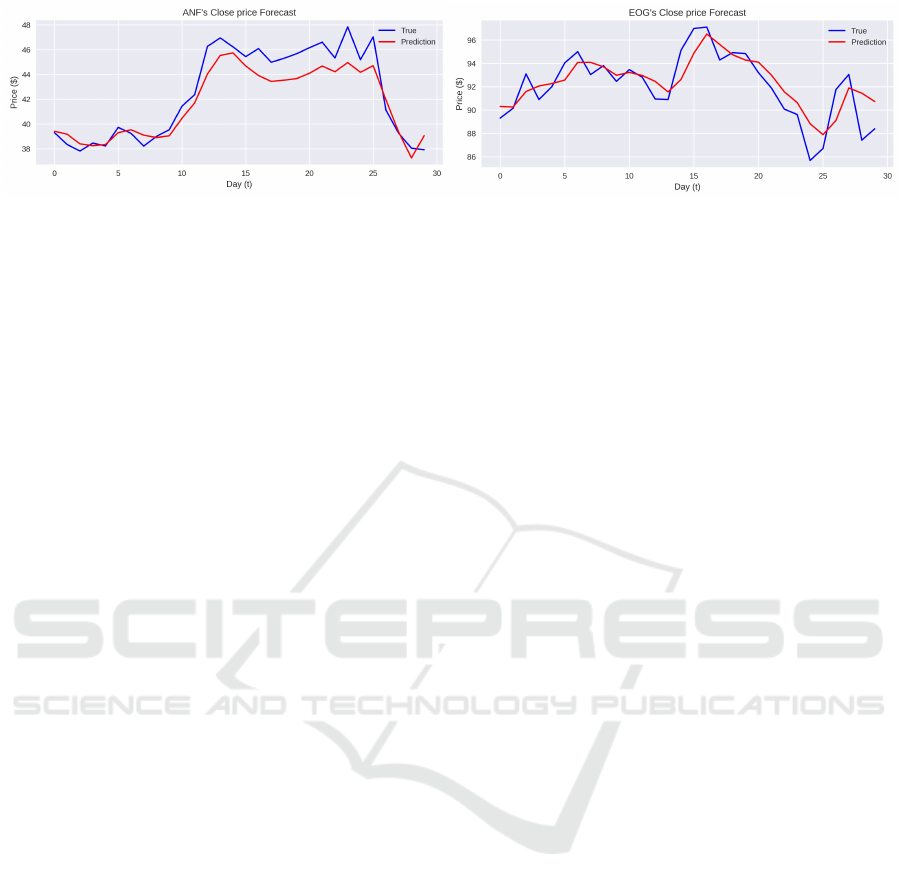
Figure 8: Detail of DNN forecast for the last 30 days of the ANF (left) and EOG (right) stock closing prices.

erage Directional Index (ADX). We also tested some

further meaningful combinations of the above indica-

tors, like in (Prasad et al., 2022), and (Hryshko and

Downs, 2004), such as ST+MO+MACD, PO+W%R

and PO+RSI.

We performed a forwardtesting of the strategies

based on each of the above indicators on the the 30-

days price forecasts following the training date ending

on October 16th, 2021, generated by the DNNs devel-

oped in Section 4.

Our results show that the best indicator for ANF is

the Triple Exponential Moving Average, whereas the

Average Directional Index is more suitable for EOG.

The corresponding trading rules, based on such indi-

cators, are shown in Figure 9, where (o), (h), (l), (c)

refer to the OHLC prices, respectively, and x is the

current (opening, highest, etc.) price. Such rules were

applied to the possible future during the forwardtest-

ing.

Then, we evaluated the proﬁt deriving from the

application of such a strategy on the real data of the

30-day trading period following October 16th, 2021,

having as starting point a budget of $100 invested in

compound mode. The results are shown in Table 7.

In particular, the evaluation is based on the following

proﬁt and risk metrics:

• Total Return (TR)

• Expectancy Ratio (ExR): measures the expected

proﬁt or loss after taking into consideration all the

past trades and their wins and losses (Investope-

dia, 2022a);

• Sharpe Ratio (ShR): a risk-adjusted proﬁt mea-

sure, which refers to the return per unit of volatil-

ity (Investopedia, 2022c);

• Sortino Ratio (SoR): a variant of the risk-adjusted

Sharpe ratio that differentiates harmful volatility

from total overall volatility by using the draw-

down as a risk measure (Investopedia, 2022d);

• Calmar Ratio (CaR): another variant of risk-

adjusted proﬁt measure, which uses the maximum

drawdown as risk measure (Investopedia, 2022b).

As a baseline to compare such metrics, we re-

evaluated the same set of technical indicators through

the traditional backtesting technique on the historical

data for the 30 days before October 16th, 2021, to

see if it would result in different choices and maybe

different proﬁts. The results show that a trader using

backtesting would choose ADX for the EOG share, as

with our forwardtesting technique, so the proﬁt would

be the same in this case. However, the TEMA in-

dicator would not be chosen for the ANF share. In-

deed, the most promising indicator, given the past 30

days of market, would be RSI (with overbought 70

and oversell 30). However, if applied to the future, it

would result in a loss of 1.16%, as shown in Table 8.

6 CONCLUSIONS

In this paper we propose a stock market trading sys-

tem that exploits deep neural networks as part of

its main components, improving the previous works

(Letteri et al., 2022a; Letteri et al., 2022b).

In such a system, the trades are guided by the

values of a pre-selected technical indicator, as usual

in algorithmic trading. However, the novelty of the

presented approach is in the indicator selection tech-

nique: traders usually make such a selection by back-

testing the system on the historical market data and

choosing the most proﬁtable indicator with respect

to the known past. On the other hand, in our ap-

proach, such most proﬁtable indicator is chosen by

forwardtesting it on the probable future predicted by

a deep neural network trained on the historical data.

As discussed in the paper, neural networks outper-

form the most common statistical methods in stock

price prediction: indeed, their predicted future allows

to make a very accurate selection of the indicator to

apply, which takes into account trends that would be

very difﬁcult to capture through backtesting.

To validate this claim, we applied our methodol-

ogy on two very different assets with medium volatil-

ity, and the results show that our forwardtesting-based

trading system achieves a proﬁt that is equal or higher

than the one of a traditional backtesting-based trading

system.

Given the promising potentials of this approach,

FEMIB 2023 - 5th International Conference on Finance, Economics, Management and IT Business

ANF

Entry ((x

(l)

< T EMA

(l)

) ∨(x

(h)

< T EMA

(h)

)) ∧((x

(c)

< T EMA

(c)

) ∨(x

(o)

< T EMA

(o)

))

Exit ((x

(l)

> T EMA

(l)

) ∨(x

(h)

> T EMA

(h)

)) ∧((x

(c)

> T EMA

(c)

) ∨(x

(o)

> T EMA

(o)

))

EOG

Entry (+DI > −DI) ∧(ADX > 25)

Exit (−DI > +DI) ∧(ADX > 25)

Figure 9: Trading system rules.

Table 7: Performance of the trading system for ANF and EOG stocks with forwardtesting-selected indicators.

#Trades TR ($) ExR ShR SoR CaR

ANF 3 6.126 2.112 2.194 3.340 12.403

EOG 3 1.374 0.525 1.253 2.556 5.814

Table 8: Performance of the trading system for ANF stock with backtesting-selected indicator (RSI).

#Trades TR ($) ExR ShR SoR CaR

ANF 1 -1.168 -1.1683 0.119 0.158 -0.935

we will further test its reliability on other stock mar-

kets using different data, such as cryptocurrencies or

deﬁ-tokens, also varying the timeframes for day trad-

ing and scalping activities. To this aim, we will also

pre-proccess the data with more reﬁned feature selec-

tion (e.g., (Letteri et al., 2020a; Letteri et al., 2019a))

and balancing (buy, sell and hold trades) (e.g., (Letteri

et al., 2020b; Letteri et al., 2021)) strategies.

We also plan to investigate the use of different,

more complex neural networks, such as Recurrent

Neural Networks or Long Short-Term Memory, that

may further improve the forecasting and therefore the

entire forwardtesting. Finally, since such neural net-

works can be seen as black-box decision-making sys-

tems, we may also investigate machine ethics moni-

toring and rules (Dyoub et al., 2021b; Dyoub et al.,

2022; Dyoub et al., 2021a) related to their activity,

and in particular the way they may inﬂuence the mar-

ket with their forecasts, if widely applied to derive

trading strategies.

REFERENCES

Akaike, H. (1974). A new look at the statistical model iden-

tiﬁcation. IEEE Transactions on Automatic Control,

19(6):716–723.

Barnwal, A., Bharti, H. P., Ali, A., and Singh, V. (2019).

Stacking with neural network for cryptocurrency in-

vestment. In 2019 New York Scientiﬁc Data Summit

(NYSDS), pages 1–5.

Danyliv, O., Bland, B., and Argenson, A. (2019). Random

walk model from the point of view of algorithmic trad-

ing.

Day, M.-Y. and Lee, C.-C. (2016). Deep learning for ﬁ-

nancial sentiment analysis on ﬁnance news providers.

2016 IEEE/ACM International Conference on Ad-

vances in Social Networks Analysis and Mining

(ASONAM), pages 1127–1134.

DHI Solution Software (2022). tsod: Anomaly detection

for time series data. https://github.com/DHI/tsod.

Dyoub, A., Costantini, S., and Letteri, I. (2022). Care robots

learning rules of ethical behavior under the supervi-

sion of an ethical teacher (short paper). In Bruno,

P., Calimeri, F., Cauteruccio, F., Maratea, M., Ter-

racina, G., and Vallati, M., editors, Joint Proceed-

ings of the 1st International Workshop on HYbrid

Models for Coupling Deductive and Inductive ReA-

soning (HYDRA 2022) and the 29th RCRA Workshop

on Experimental Evaluation of Algorithms for Solv-

ing Problems with Combinatorial Explosion (RCRA

2022) co-located with the 16th International Confer-

ence on Logic Programming and Non-monotonic Rea-

soning (LPNMR 2022), Genova Nervi, Italy, Septem-

ber 5, 2022, volume 3281 of CEUR Workshop Pro-

ceedings, pages 1–8. CEUR-WS.org.

Dyoub, A., Costantini, S., Letteri, I., and Lisi, F. A. (2021a).

A logic-based multi-agent system for ethical monitor-

ing and evaluation of dialogues. In Formisano, A.,

Liu, Y. A., Bogaerts, B., Brik, A., Dahl, V., Dodaro,

C., Fodor, P., Pozzato, G. L., Vennekens, J., and Zhou,

N., editors, Proceedings 37th International Confer-

ence on Logic Programming (Technical Communica-

tions), ICLP Technical Communications 2021, Porto

(virtual event), 20-27th September 2021, volume 345

of EPTCS, pages 182–188.

Dyoub, A., Costantini, S., Lisi, F. A., and Letteri, I. (2021b).

Ethical monitoring and evaluation of dialogues with

a mas. In Monica, S. and Bergenti, F., editors, Pro-

ceedings of the 36th Italian Conference on Compu-

tational Logic, Parma, Italy, September 7-9, 2021,

volume 3002 of CEUR Workshop Proceedings, pages

158–172. CEUR-WS.org.

Facebook Open Source (2022). Prophet github pages. https:

//facebook.github.io/prophet/.

Global Newswire (2021). Abercrombie & ﬁtch

co. reports third quarter results. https:

//www.globenewswire.com/news-release/2021/11/

Trading Strategy Validation Using Forwardtesting with Deep Neural Networks

23/2339734/0/en/Abercrombie-Fitch-Co-Reports-

Third-Quarter-Results.html.

Hansen, J. V., McDonald, J. B., and Nelson, R. D. (1999).

Time series prediction with genetic-algorithm de-

signed neural networks: An empirical comparison

with modern statistical models. Computational Intel-

ligence, 15(3):171–184.

Hinton, G. E., Srivastava, N., Krizhevsky, A., Sutskever,

I., and Salakhutdinov, R. (2012). Improving neural

networks by preventing co-adaptation of feature de-

tectors. CoRR, abs/1207.0580.

Hryshko, A. and Downs, T. (2004). System for foreign

exchange trading using genetic algorithms and rein-

forcement learning. International Journal of Systems

Science, 35(13-14):763–774.

Investopedia (2019). 3 oil and gas stocks to watch this

week. https://www.investopedia.com/3-oil-and-gas-

stocks-to-watch-this-week-4628357.

Investopedia (2020). Buy and hold deﬁnition. https://www.

investopedia.com/terms/b/buyandhold.asp.

Investopedia (2022a). Break-even analysis. https://www.

investopedia.com/terms/b/breakevenanalysis.asp.

Investopedia (2022b). Calmar ratio. https://www.

investopedia.com/terms/c/calmarratio.asp.

Investopedia (2022c). Sharpe ratio. https://www.

investopedia.com/terms/s/sharperatio.asp.

Investopedia (2022d). Sortino ratio. https://www.

investopedia.com/terms/s/sortinoratio.asp.

Krizhevsky, A., Sutskever, I., and Hinton, G. E. (2012).

Imagenet classiﬁcation with deep convolutional neu-

ral networks. In Proceedings of the 25th Interna-

tional Conference on Neural Information Processing

Systems - Volume 1, NIPS’12, page 1097–1105, Red

Hook, NY, USA. Curran Associates Inc.

Kumbure, M. M., Lohrmann, C., Luukka, P., and Porras,

J. (2022). Machine learning techniques and data for

stock market forecasting: A literature review. Expert

Systems with Applications, 197:116659.

Lee, T.-S. and Chiu, C.-C. (2002). Neural network fore-

casting of an opening cash price index. International

Journal of Systems Science, 33(3):229–237.

Letteri, I., Della Penna, G., and Caianiello, P. (2019a). Fea-

ture selection strategies for HTTP botnet trafﬁc de-

tection. In 2019 IEEE European Symposium on Se-

curity and Privacy Workshops, EuroS&P Workshops

2019, Stockholm, Sweden, June 17-19, 2019, pages

202–210. IEEE.

Letteri, I., Della Penna, G., and De Gasperis, G. (2018).

Botnet detection in software deﬁned networks by deep

learning techniques. In Castiglione, A., Pop, F., Ficco,

M., and Palmieri, F., editors, Cyberspace Safety and

Security - 10th International Symposium, CSS 2018,

Amalﬁ, Italy, October 29-31, 2018, Proceedings, vol-

ume 11161 of Lecture Notes in Computer Science,

pages 49–62. Springer.

Letteri, I., Della Penna, G., and De Gasperis, G. (2019b).

Security in the internet of things: botnet detec-

tion in software-deﬁned networks by deep learning

techniques. Int. J. High Perform. Comput. Netw.,

15(3/4):170–182.

Letteri, I., Della Penna, G., De Gasperis, G., and Dyoub, A.

(2022a). A stock trading system for a medium volatile

asset using multi layer perceptron.

Letteri, I., Della Penna, G., Di Vita, L., and Grifa, M. T.

(2020a). Mta-kdd’19: A dataset for malware traf-

ﬁc detection. In Loreti, M. and Spalazzi, L., editors,

Proceedings of the Fourth Italian Conference on Cy-

ber Security, Ancona, Italy, February 4th to 7th, 2020,

volume 2597 of CEUR Workshop Proceedings, pages

153–165. CEUR-WS.org.

Letteri, I., Di Cecco, A., and Della Penna, G. (2020b).

Dataset optimization strategies for malware trafﬁc de-

tection. CoRR, abs/2009.11347.

Letteri, I., Di Cecco, A., Dyoub, A., and Della Penna, G.

(2021). Imbalanced dataset optimization with new re-

sampling techniques. In Arai, K., editor, Intelligent

Systems and Applications - Proceedings of the 2021

Intelligent Systems Conference, IntelliSys 2021, Am-

sterdam, The Netherlands, 2-3 September, 2021, Vol-

ume 2, volume 295 of Lecture Notes in Networks and

Systems, pages 199–215. Springer.

Letteri, I., Penna, G. D., Gasperis, G. D., and Dyoub, A.

(2022b). Dnn-forwardtesting: A new trading strat-

egy validation using statistical timeseries analysis and

deep neural networks. CoRR, abs/2210.11532.

Linke, A., Mash, L., Fong, C., Kinnear, M., Kohli, J.,

Wilkinson, M., Tung, R., Jao Keehn, R., Carper, R.,

Fishman, I., and Müller, R.-A. (2020). Dynamic time

warping outperforms pearson correlation in detecting

atypical functional connectivity in autism spectrum

disorders. NeuroImage, 223:117383.

Lu, J. and Ohta, H. (2002). Using the optimization layer-

by-layer learning algorithm on local-recurrent-global-

feedforward networks in ﬁnancial time series pre-

dictions. International Journal of Systems Science,

33(12):959–967.

Marín, G., Caasas, P., and Capdehourat, G. (2021). Deep-

mal - deep learning models for malware trafﬁc detec-

tion and classiﬁcation. In Haber, P., Lampoltshammer,

T., Mayr, M., and Plankensteiner, K., editors, Data

Science – Analytics and Applications, pages 105–112,

Wiesbaden. Springer Fachmedien Wiesbaden.

Marquez, J. (1995). Time series analysis : James d. hamil-

ton, 1994, (princeton university press, princeton, nj).

International Journal of Forecasting, 11(3):494–495.

Mehra, R. (1998). On the volatility of stock prices: an ex-

ercise in quantitative theory. International Journal of

Systems Science, 29(11):1203–1211.

Mondal, S. S., Mohanty, S. P., Harlander, B., Koseoglu,

M., Rane, L., Romanov, K., Liu, W.-K., Hatwar,

P., Salathe, M., and Byrum, J. (2019). Investment

Ranking Challenge: Identifying the best performing

stocks based on their semi-annual returns. Papers

1906.08636, arXiv.org.

Prasad, P. S. K., Madhav, V., Lal, R., and Ravi, V. (2022).

Optimal technical indicator-based trading strategies

using nsga-ii.

scikit-learn (2022). Gridsearchcv. https://scikit-

learn.org/stable/modules/generated/sklearn.model\

_selection.GridSearchCV.html.

FEMIB 2023 - 5th International Conference on Finance, Economics, Management and IT Business

Smith, T. G. (2022). pmdarima: Arima estimators

for python. https://alkaline-ml.com/pmdarima/setup.

html.

Sokolov, A. N., Alabugin, S. K., and Pyatnitsky, I. A.

(2019). Trafﬁc modeling by recurrent neural networks

for intrusion detection in industrial control systems.

In 2019 International Conference on Industrial Engi-

neering, Applications and Manufacturing (ICIEAM),

pages 1–5.

Soniya, Paul, S., and Singh, L. (2015). A review on ad-

vances in deep learning. 2015 IEEE Workshop on

Computational Intelligence: Theories, Applications

and Future Directions (WCI), pages 1–6.

Stoica, P. and Selen, Y. (2004). Model-order selection: a re-

view of information criterion rules. IEEE Signal Pro-

cessing Magazine, 21(4):36–47.

Tsantekidis, A., Passalis, N., Tefas, A., Kanniainen, J., Gab-

bouj, M., and Iosiﬁdis, A. (2017). Forecasting stock

prices from the limit order book using convolutional

neural networks. In 2017 IEEE 19th Conference on

Business Informatics (CBI), volume 01, pages 7–12.

Žuni

c, E., Korjeni

c, K., Hodži

c, K., and Ðonko, D. (2020).

Application of facebook’s prophet algorithm for suc-

cessful sales forecasting based on real-world data. In-

ternational Journal of Computer Science and Infor-

mation Technology, 12(2):23–36.

Yahoo Finance (2020). Anf stock price data. https://it.

ﬁnance.yahoo.com/quote/ANF.

Yao, J., Tan, C. L., and Poh, H.-L. (1999). Neural networks

for technical analysis: a study on klci. International

journal of theoretical and applied ﬁnance, 2(02):221–

241.

Trading Strategy Validation Using Forwardtesting with Deep Neural Networks