Visual Looming from Motion Field and Surface Normals
Juan D. Yepes and Daniel Raviv
Florida Atlantic University,
Electrical Engineering and Computer Science Department,
Keywords:
Looming, Obstacle Avoidance, Collision Free Navigation, Motion Field, Optical Flow, Threat Zones,
Autonomous Vehicles.
Abstract:
Looming, traditionally defined as the relative expansion of objects in the observer’s retina, is a fundamental
visual cue for perception of threat and can be used to accomplish collision free navigation. In this paper we
derive novel solutions for obtaining visual looming quantitatively from the 2D motion field resulting from a
six-degree-of-freedom motion of an observer relative to a local surface in 3D. We also show the relationship
between visual looming and surface normals. We present novel methods to estimate visual looming from
spatial derivatives of optical flow without the need for knowing range. Simulation results show that estimations
of looming are very close to ground truth looming under some assumptions of surface orientations. In addition,
we present results of visual looming using real data from the KITTI dataset. Advantages and limitations of the
methods are discussed as well.
1 INTRODUCTION
The visual looming cue, defined quantitatively by
(Raviv, 1992) as the negative instantaneous change
of range over the range, is related to the increase in
size of an object projected on the observer’s retina.
Visual looming can be used to define threat regions
for obstacle avoidance without the need of range and
image understanding. Visual looming is independent
of camera rotation and can indicate threat of moving
objects as well.
Studies in biology have shown strong evidence
of neural circuits in the brains of creatures related
to the identification of looming (Ache et al., 2019).
Basically, creatures have instinctive escaping behav-
iors that tie perception directly to action. This way
creatures can avoid impending threat from predators
that project an expanding image on their visual sys-
tems (Evans et al., 2018)(Yilmaz and Meister, 2013).
Also, there is evidence of looming being involved in
specialized behaviors, for example controlling the ac-
tion prior to an imminent collision with water surface
as exhibited by plummeting gannets (Lee and Red-
dish, 1981) or acrobatic evasive maneuvers exhibited
by flies (Fabian et al., 2022)(Muijres et al., 2014).
According to Gibson (Gibson, 2014), motion rel-
ative to a surface is one of the most fundamental vi-
sual perceptions. He argued that visual information
is processed in a bottom up way, starting from simple
to more complex processing. The perceived optical
flow resulting from motion of the observer is suffi-
cient to make sense of the environment where a direct
connection from visual perception to action can be es-
tablished. Optical flow analysis is a primitive, simple
and robust method for various visual tasks such as dis-
tance estimation, image segmentation, surface orien-
tation and object shape estimation (Albus and Hong,
1990)(Cipolla and Blake, 1992).
Optical flow is the estimation of the motion field,
which is the 2D perspective projection on the image
of the true 3D velocity field as a consequence of the
observer’s relative motion. Optical flow can be cal-
culated using a number of algorithms that process
variations of patterns on image brightness (Horn and
Schunck, 1981)(Verri and Poggio, 1986)(Zhai et al.,
2021).
Optical flow measurements, as the estimation
of motion field, includes the necessary information
about the relative rate of expansion of objects between
two consecutive images from which the visual loom-
ing cue can be estimated (Raviv, 1992).
In this paper, we present two novel analyti-
cal closed form expressions for calculating looming
for any six-degree-of-freedom motion, using spatial
derivatives of the motion field. The approach can be
applied to any relative motion of the camera and any
46
Yepes, J. and Raviv, D.
Visual Looming from Motion Field and Surface Normals.
DOI: 10.5220/0011727400003479
In Proceedings of the 9th International Conference on Vehicle Technology and Intelligent Transport Systems (VEHITS 2023), pages 46-53
ISBN: 978-989-758-652-1; ISSN: 2184-495X
Copyright
c
 2023 by SCITEPRESS – Science and Technology Publications, Lda. Under CC license (CC BY-NC-ND 4.0)

F
V
z
x
y
F
> >
a)
b)
Object
at time t1
Object
at time t2
Visual images
at times t1 and t2
Relative
velocity
Figure 1: Visualizing looming cue: a) relative expansion of
3D object on spherical image, b) equal looming spheres as
shown for a given translation
ˆ
t.
visible surface point. In addition, we show the theo-
retical relationship between the value of looming and
surface orientation. In simulation results we show the
effect of the surface normal to the accuracy of the es-
timated looming values. We demonstrate a new way
to extract looming from optical flow using the RAFT
model and derived relevant expressions. We show
that egomotion is not required for estimating loom-
ing. In other words, knowledge of range to the point,
as well as relative translation or rotation information
are not required for computing looming and hence for
autonomous navigation tasks.
2 RELATED WORK
2.1 Visual Looming
The visual looming cue is related to the relative
change in size of an object projected on the observer’s
retina as the range to the object increases (Figure 1.a).
It is defined quantitatively as the negative value of the
time derivative of the range between the observer and
a point in 3D divided by the range (Raviv, 1992):
L = − lim
∆t→0

r
2
−r
1
∆t

r
1
(1)
L = −

˙r
r

(2)
where L denotes looming, t
1
represents time instance
1, t
2
represents time instance 2, ∆t is t
2
−t
1
, r
1
is the
range to the point at time instance t
1
, and r
2
is the
range at time instance t
2
. Dot denotes derivative with
respect to time.
Please note that in this paper we use the terms
camera, observer and vehicle interchangeably.
Figure 2: Looming spheres: a) Looming spheres superim-
posed on vehicle trajectory; b) for given identical looming
values b1 shows the looming spheres for low speed and b2
shows the looming spheres for high speed.
2.1.1 Looming Properties
Note that the result for L in equation (2) is a scalar
value. L is dependent on the vehicle translation com-
ponent but independent of the vehicle rotation. Also
L is measured in [time
−1
] units.
It was shown that points in space that share the
same looming values form equal looming spheres
with centers that lie on the instantaneous translation
vector t and intersect with the vehicle origin. These
looming spheres expand and contract depending on
the magnitude of the translation vector (Raviv, 1992).
Since an equal looming sphere corresponds to a
particular looming value, there are other spheres with
varying values of looming with different radii. A
smaller sphere signifies a higher value of looming as
shown in Figure 1.b (L
3
> L
2
> L
1
).
Regions for obstacle avoidance and other
behavior-related tasks can be defined using equal
looming spheres. For example, a high danger zone
for L > L
3
, medium threat for L
3
> L > L
2
and low
threat for L
2
> L > L
1
.
2.1.2 Advantages of Looming
Looming provides time-based imminent threat to the
observer caused by stationary environment or moving
objects (Raviv, 1992). There is no need for scene un-
derstanding such as identifying cars, bikes or pedes-
trians. Threat regions can be obtained from looming
values by assigning specific thresholds. Figure 2.a
shows the looming sphere as a function of time for a
given constant speed. For the same identical values of
looming L
1
, L
2
and L
3
, Figure 2.b shows equal loom-
ing spheres using two (time based) threat zones. Fig-
ure 2.b1 shows looming spheres at low speed and Fig-
ure 2.b2 shows looming spheres at high speed. Note
that the radii of the spheres are proportional to the
speed of the vehicle.
Visual looming can provide indication of threat
from moving objects as shown in Figure 3. Threats
from approaching objects are visualized as bright red
colors while receding objects appear in blue.
Visual Looming from Motion Field and Surface Normals
47

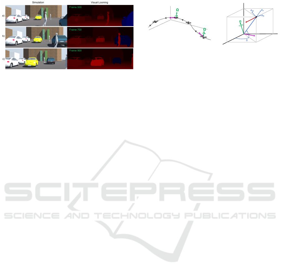
Figure 3: Visual Looming from Simulation: left - a image
sequence of the simulated scene. Note that the white and
yellow cars are approaching the observer and the blue car is
moving away from the observer; right - the corresponding
looming values for the image sequence (the brighter the red
the higher the threat; blue corresponds to negative looming).
2.1.3 Measuring Visual Looming
Several methods were shown to quantitatively extract
the visual looming cue from a 2D image sequence by
measuring attributes like area, brightness, texture den-
sity and image blur (Raviv and Joarder, 2000).
Similar to visual looming, the Visual Threat Cue
(VTC) is a measurable time-based scalar value that
provides some measure for a relative change in range
between a 3D surface and a moving observer (Kundur
and Raviv, 1999). Event-based cameras were shown
to detect looming objects in real-time from optical
flow (Ridwan, 2018).
2.2 Motion Field and Optical Flow
Motion field is the 2D projection of the true 3D veloc-
ity field onto the image surface while the optical flow
is the local apparent motion of points in the image
(Verri and Poggio, 1986). Basically, optical flow is an
estimation of the motion field that can be recovered
using a number of algorithms that exploit the spatial
and temporal variations of patterns of image bright-
ness (Horn and Schunck, 1981). From the computer
vision perspective the question is how to obtain infor-
mation about the camera motion and objects in the en-
vironment from estimations of the motion field (Aloi-
monos, 1992). Optical flow algorithms are divided in
three categories: knowledge driven, data driven and
hybrid. A comprehensive survey of optical flow and
scene flow estimation algorithms were provided by
(Zhai et al., 2021).
In this paper we make use of a state of the art
approach to compute optical flow called RAFT
(Recurrent all-pairs field transforms for optical flow)
(Teed and Deng, 2020) which we use as a given input
to our method to obtain estimations of visual looming.
z
x
y
t
t
z
x
y
r
t
F
V
ϕ
a)
b)
Figure 4: General motion of a vehicle in 3D space. a) Vehi-
cle trajectory in world coordinates with translation vector t
and rotation vector Ω. b) Camera coordinate system.
Estimation of optical flow from a sequence of
images is beyond the scope of this paper.
3 METHOD
In this section we derive two different expressions
for visual looming (L) for a general six-degrees-of-
freedom motion. As mentioned earlier, the camera is
attached to the vehicle and both share the same coor-
dinate system.
3.1 Velocity and Motion Fields
Consider a vehicle motion in 3D space relative to an
arbitrary stationary reference point F (refer to Figure
4). At any given time, the vehicle velocity vector con-
sists of a translation component t and a rotation com-
ponent Ω in world coordinates as shown in Figure 4.a.
Also consider a local coordinate system centered at
the camera which is fixed to the moving vehicle (Fig-
ure 4.b). We choose the z-axis to be aligned with the
vertical orientation of the camera and the x-axis to
be aligned with the optical axis of the camera. In this
frame any stationary point in the 3D scene can be rep-
resented using spherical coordinates (r,θ,φ) where r
is the range to the point F, θ is the azimuth angle mea-
sured from the x-axis and φ is the elevation angle from
the XY-plane.
In camera coordinates, a point F has an associated
relative velocity V with a translation vector −t and ro-
tation vector −Ω, given by (see (Meriam and Kraige,
2012)):
V = (−t) + (−Ω × r) (3)
Note that r in bold refers to the range vector and the
scalar r refers to its magnitude, i.e., r = |r|. Notice
also that for a given point F, the velocity vector V is
the velocity field in 3D due to egomotion of the cam-
era.
By dividing equation (3) by the scalar r and
expanding t and Ω we get:
VEHITS 2023 - 9th International Conference on Vehicle Technology and Intelligent Transport Systems
48

V
r
=

−t
r

+

−Ω × r
r

=
−(t
r
e
r
+t
θ
e
θ
+t
φ
e
φ
)
r
− (Ω
r
e
r
+ Ω
θ
e
θ
+ Ω
φ
e
φ
) × e
r
=

−t
r
r

e
r
+

−t
θ
r

e
θ
+

−t
φ
r

e
φ
+ (−Ω
φ
)e
θ
+ Ω
θ
e
φ
(4)
where:
t
r
= t · e
r
, Ω
r
= Ω · e
r
t
θ
= t · e
θ
, Ω
θ
= Ω · e
θ
t
φ
= t · e
φ
, Ω
φ
= Ω · e
φ
The velocity field V can also be expressed in
spherical coordinates (r,θ,φ) and directional unit vec-
tors (e
r
,e
θ
,e
φ
) as shown in (Meriam and Kraige,
2012):
V = ˙re
r
+ r
˙
θcos(φ)e
θ
+ r
˙
φe
φ
(5)
By dividing equation (5) by r we obtain:
V
r
=

˙r
r

e
r
+
˙
θcos(φ)e
θ
+
˙
φe
φ
(6)
From (6) we can identify the 2D motion field f defined
as:
f =
˙
θcos(φ)e
θ
+
˙
φe
φ
(7)
Note that

˙r
r

is not part of the motion field since
it is along the range direction e
r
from the camera to
point F. The motion field f in expression (7) is the
projection of the velocity field V on the spherical im-
age.
3.2 Looming from Spatial Partial
Derivatives of the Velocity Field
The Looming value (L) is related to the relative ex-
pansion of objects projected on the image of the cam-
era. This means that there is a direct relationship be-
tween the change in the motion field in the vicinity of
a point and looming (L). In order to find this relation-
ship we apply spatial partial derivatives with respect
to θ and φ to the velocity field divided by r as de-
scribed in equations (4) and (6) to get:
∂
∂θ

V
r

=
∂
∂θ

−t
r
r

e
r
+

−t
θ
r

e
θ
+

−t
φ
r

e
φ

+
∂
∂θ

(−Ω
φ
)e
θ
+ Ω
θ
e
φ

=
∂
∂θ

˙r
r

e
r
+
˙
θcos(φ)e
θ
+
˙
φe
φ

(8)
∂
∂φ

V
r

=
∂
∂φ

−t
r
r

e
r
+

−t
θ
r

e
θ
+

−t
φ
r

e
φ

+
∂
∂φ

(−Ω
φ
)e
θ
+ Ω
θ
e
φ

=
∂
∂φ

˙r
r

e
r
+
˙
θcos(φ)e
θ
+
˙
φe
φ

(9)
By performing the corresponding derivations
1
for
equations (8) and (9), in addition to using equation
(2) for L, we obtain the following two independent
expressions for looming (L):
L =
∂
˙
θ
∂θ
−
˙
φtan(φ)−
t
θ
r

1
cos(φ)

1
r
∂r
∂θ

(10)
L =
∂
˙
φ
∂φ
−
t
φ
r

1
r
∂r
∂φ

(11)
In both expressions, L is a scalar value that can be
computed from the spatial change in the motion field.
Note that L is independent of the vehicle rotation Ω
and is dependent only on the translation components
scaled by r, t
θ
/r and t
φ
/r.
These expressions may also apply to any rela-
tive motion of a point in 3D for any six-degrees-of-
freedom motion.
3.3 Estimation of Visual Looming
Expressions (10) and (11) contain r, which is not mea-
surable from the image. If we estimate looming by
eliminating the components that contain r in (10) and
(11) then estimates for L are obtained as:
L
est1
=
∂
˙
θ
∂θ
−
˙
φtanφ (12)
L
est2
=
∂
˙
φ
∂φ
(13)
Later in the paper, we show the effect of eliminat-
ing the components in equations (12) and (13) that
include r and its derivative on the error in calculating
looming.
Notice that L
est1
and L
est2
can be obtained di-
rectly from measurements of the horizontal and ver-
tical components of the motion field for a particular
time instance, specifically, the changes of the values
of the motion field in the spatial dimensions θ and φ.
This is the meaning of the spatial partial derivatives
∂
˙
θ
∂θ
,
∂
˙
φ
∂φ
in expressions (12) and (13).
1
Most of the detailed derivations were omitted from the
paper due to page limit. The detailed derivations are avail-
able upon request.
Visual Looming from Motion Field and Surface Normals
49

Figure 5: Surface orientation: a) infinitesimal planar surface
represented by the triangle ABC; b) tilt angles related to the
normal of the planar patch
3.4 Surface Normals
The point F lies on a infinitesimally small surface
patch with normal vector n. To find the relation be-
tween L and n we assume that the surface is planar
in the vicinity of the point. This planar patch is rep-
resented by the triangle ABC and n is the normal at
point F (see Figure 5.a).
We can identify two vectors,
∂r
∂θ
and
∂r
∂φ
, located on
the planar patch, that result from the displacement of r
along the angles θ and φ. Notice that these vectors are
both perpendicular to the surface normal n and are lo-
cated at the intersection of the planes ABC, e
r
e
φ
, and
e
θ
e
φ
. It can be shown that the following constraints
hold for any infinitesimal small patch:
∂r
∂θ
· n = 0 (14)
∂r
∂φ
· n = 0 (15)
Using r = re
r
and solving for
∂r
∂θ
and
∂r
∂φ
in (14) and
(15) we obtain:
1
r
∂r
∂θ
= −cos φ

e
θ
· n
e
r
· n

(16)
1
r
∂r
∂φ
= −

e
φ
· n
e
r
· n

(17)
By defining the surface tilt angles as γ and δ (see Fig-
ure 5.b) we obtain:
γ = tan
−1

e
θ
· n
e
r
· n

(18)
δ = tan
−1

e
φ
· n
e
r
· n

(19)
We can rewrite equations (10), (11) using (16), (17),
(18) and (19) as:
a)
b)
c)
Figure 6: Simulation of a vehicle moving in 3D space and
a point on a planar patch. a) Vehicle trajectory. b) Motion
parameters t and Ω.
L =
∂
˙
θ
∂θ
−
˙
φtan φ +

t
θ
r

tanγ (20)
L =
∂
˙
φ
∂φ
+

t
φ
r

tanδ (21)
Equations (20) and (21) are essentially the same as
expressions (10) and (11) but using normal notations.
4 LOOMING RESULTS
We present two sets of quantitative results of the
methods for estimation of looming using simulations
and real data.
4.1 Looming from Simulation
We simulated a translating and rotating observer in
3D. Measurements were taken for a single stationary
point on a tilted planar patch (see Figure 6.a).
The simulation duration was 23 seconds and sam-
ples were taken at 60 Hz (1380 samples in total).
The vehicle starting position was P = −75i + 75j +
44.3k and the orientation was [forward, left, up] =
[−i,−j,k]. The planar patch was simulated by the fol-
lowing points: A = 80i − 40j + 40k, B = 80i − 80j +
35k and C = 85i − 60j + 58k. All distances were in
meters. The vehicle was moving at a speed of s =
11.11 m/s (or 40 km/h) with translation and rotation
vectors t = si + 0.1s cos(0.1t)j + 0.1s cos(0.2t)k and
Ω = cos(0.1t)i − cos(0.3t)j + 8(
π
180
)sin(0.3t)k.
Plots of the parameters t and Ω over time are
shown on Figure 6.b.
Ground truth looming L is computed from range
and its time derivative using equation (1). In addition,
two estimations of looming L
1
and L
2
are computed
using equations (20) and (21) (see Figure 7). To com-
pare L with each estimate of L
1
or L
2
we use the error
percentage metric:
error
i
(%) =
L
i
− L
L
× 100 for i = 1,2 (22)
VEHITS 2023 - 9th International Conference on Vehicle Technology and Intelligent Transport Systems
50

Figure 7: Ground truth looming (L) and estimated looming
(L
1
and L
2
).
Figure 8: Left: error percentage (error
1
, error
2
) between
ground truth L and estimated looming values L
1
, L
2
. Right:
tilt angles γ and δ related to the normal of the planar patch.
Plots, as a function of time, for both error values:
error
1
and error
2
that correspond to L
1
and L
2
are
shown in Figure 8 (left). In Figure 8 (right), values
of the tilt angles of the planar patch γ and δ are pre-
sented.
Notice that for this particular simulation, L
2
val-
ues are closer to L than L
1
values. This can be ex-
plained by a smaller value of the tilt angle δ which
introduces less estimation error. The discontinuity in
the error signal plot (around time = 17.2s) is due to L
becoming closer to zero in equation (22).
For example, in Figure 8 the ground truth looming
has a positive maximum L = 0.129s
−1
at t = 13.8s,
and the estimated values are L
1
= 0.147s
−1
, and L
2
=
0.117s
−1
. Both estimates get very close to the ground
truth of L with error
1
= 13% and error
2
= −9%.
This simulation shows that when tilt angles are
small (lower than ±20 degrees) the error in the es-
timation of looming is within ±15% range. Un-
der these assumptions looming estimates are good
enough to define threat zones for collision avoidance
tasks where thresholds can be adjusted by this margin
of error.
4.2 Looming from Real Data
Visual looming estimates were obtained from optical
flow (estimation of the motion field) from a sequence
of images taken from a moving camera fixed on a ve-
hicle. The block diagram in Figure 9 shows the pro-
cess and the different components.
Figure 9: Estimation of looming using real data.
Figure 10: Estimated Looming from KITTI. a) Original im-
ages (frame 69 and frame 70), b) Optical flow estimate from
RAFT. c) Estimated Looming using the average value from
equations (12) and (13).
We processed real data using a particular city drive
from the well known KITTI dataset (Geiger et al.,
2013). This dataset includes raw data from several
sensors mounted on a vehicle. We used a video se-
quence from one of the color cameras (FL2-14S3C-
C, 1.4 Megapixels, 1392x512 pixels). Then a pair of
consecutive RGB images from this dataset were pro-
cessed by a deep neural network called RAFT (Re-
current All-Pairs Field Transforms) (Teed and Deng,
2020). RAFT provides optical flow estimation as out-
put, for each pixel in the image as a displacement
pixel pair (u,v).
We used the KITTI camera intrinsic parameters
to transform from pixel image coordinates to spheri-
cal coordinates and obtained (θ,φ,
˙
θ,
˙
φ). Then the av-
erage of spatial derivatives from equations (12) and
(13) were applied to estimate and visualize the loom-
ing values.
Looming estimation from frames 69 and 70 are
shown in Figure 10.c. Positive values of looming are
shown in red and negative values in blue. The brighter
the red, the higher the looming threat.
Notice an edge effect around objects with high
values of red and blue colors. This is due to occlu-
sions that generate sudden changes in optical flow and
cause distortion of looming, resulting in incorrect val-
ues. Those may be managed by discarding some blue
regions using additional filtering.
Notice also some noise, shown as square artifacts,
due the up-sampling interpolation stage of the RAFT
Visual Looming from Motion Field and Surface Normals
51

algorithm (1:8 ratio). The noise is due to spatial par-
tial derivatives that have a tendency to amplify minor
differences of optical flow.
Moving objects, like the bike and the white car in
the image sequence, are shown with darker red color
(meaning less threat) due to small relative velocity
with respect to the camera. This is an advantage of the
approach where estimation of looming is able to catch
the relevant threat of moving objects. This is clearly
an advantage of looming over conventional percep-
tion of depth.
5 CONCLUSIONS
Visual looming has been shown to be an important
cue for navigation and control tasks. This paper ex-
plores new ways for deriving and estimating visual
looming for general six-degrees-of-freedom motion.
The main contributions of the paper are:
1. We derived two novel analytical closed-form ex-
pressions for calculating looming for any six-
degree-of-freedom motion. These expressions in-
clude spatial derivatives of the motion field. This
approach can be applied to any relative motion be-
tween an observer and any visible point.
2. We showed the theoretical relationship of surface
normal to the values of looming.
3. We presented simulation results of the effect of
surface normals on values of calculated looming.
Quantitative calculations showed the relationship
between the angles of the surface normal relative
to the angle of the range vector and the related
effects on the accuracy of estimating looming val-
ues.
4. We demonstrated how to extract looming from op-
tical flow. The output of the RAFT model was
used to estimate looming values using expressions
that were derived in the paper.
It should also be emphasized that knowledge of range
to the 3D point, translation or rotation of the cam-
era (egomotion) is not required for the estimation of
looming and hence for autonomous navigation tasks.
ACKNOWLEDGMENTS
The authors thank Dr. Sridhar Kundur for many fruit-
ful discussion and suggestions as well as very detailed
comments and clarifications that led to meaningful
improvements of this paper. The authors also thank
Nikita Ostro and Benjamin Thaw for their thorough
review of this paper.
REFERENCES
Ache, J. M., Polsky, J., Alghailani, S., Parekh, R., Breads,
P., Peek, M. Y., Bock, D. D., von Reyn, C. R., and
Card, G. M. (2019). Neural basis for looming size and
velocity encoding in the drosophila giant fiber escape
pathway. Current Biology, 29(6):1073–1081.
Albus, J. S. and Hong, T. H. (1990). Motion, depth, and im-
age flow. In Proceedings., IEEE International Confer-
ence on Robotics and Automation, pages 1161–1170.
IEEE.
Aloimonos, Y. (1992). Is visual reconstruction necessary?
obstacle avoidance without passive ranging. Journal
of Robotic Systems, 9(6):843–858.
Cipolla, R. and Blake, A. (1992). Surface orientation and
time to contact from image divergence and deforma-
tion. In European Conference on Computer Vision,
pages 187–202. Springer.
Evans, D. A., Stempel, A. V., Vale, R., Ruehle, S., Lefler,
Y., and Branco, T. (2018). A synaptic threshold
mechanism for computing escape decisions. Nature,
558(7711):590–594.
Fabian, S. T., Sumner, M. E., Wardill, T. J., and Gonzalez-
Bellido, P. T. (2022). Avoiding obstacles while in-
tercepting a moving target: a miniature fly’s solution.
Journal of Experimental Biology, 225(4):jeb243568.
Geiger, A., Lenz, P., Stiller, C., and Urtasun, R. (2013).
Vision meets robotics: The kitti dataset. The Inter-
national Journal of Robotics Research, 32(11):1231–
1237.
Gibson, J. J. (2014). The ecological approach to visual per-
ception: classic edition. Psychology Press.
Horn, B. K. and Schunck, B. G. (1981). Determining optical
flow. Artificial intelligence, 17(1-3):185–203.
Kundur, S. R. and Raviv, D. (1999). Novel active vision-
based visual threat cue for autonomous navigation
tasks. Computer Vision and Image Understanding,
73(2):169–182.
Lee, D. N. and Reddish, P. E. (1981). Plummeting gan-
nets: A paradigm of ecological optics. Nature,
293(5830):293–294.
Meriam, J. and Kraige, L. (2012). Engineering Mechanics:
Dynamics. Engineering Mechanics. Wiley.
Muijres, F. T., Elzinga, M. J., Melis, J. M., and Dickinson,
M. H. (2014). Flies evade looming targets by exe-
cuting rapid visually directed banked turns. Science,
344(6180):172–177.
Raviv, D. (1992). A quantitative approach to looming. US
Department of Commerce, National Institute of Stan-
dards and Technology.
Raviv, D. and Joarder, K. (2000). The visual looming nav-
igation cue: A unified approach. Comput. Vis. Image
Underst., 79:331–363.
Ridwan, I. (2018). Looming object detection with event-
based cameras. University of Lethbridge (Canada).
Teed, Z. and Deng, J. (2020). Raft: Recurrent all-pairs field
transforms for optical flow. In European conference
on computer vision, pages 402–419. Springer.
Verri, A. and Poggio, T. (1986). Motion field and optical
flow: qualitative properties.
VEHITS 2023 - 9th International Conference on Vehicle Technology and Intelligent Transport Systems
52

Yilmaz, M. and Meister, M. (2013). Rapid innate defensive
responses of mice to looming visual stimuli. Current
Biology, 23(20):2011–2015.
Zhai, M., Xiang, X., Lv, N., and Kong, X. (2021). Optical
flow and scene flow estimation: A survey. Pattern
Recognition, 114:107861.
Visual Looming from Motion Field and Surface Normals
53