The Evolution of the South-Eastern Baltic Sea Coastline Between

1988 and 2018 by Remote Sensing

Sébastien Gadal

1,2 a

and Thomas Gloaguen

1,3 b

Aix-Marseille Université, Université Côte-d’Azur, Avignon Université, CNRS, ESPACE UMR 7300,

84000 Avignon, France

Department of Ecology and Geography, Institute of Natural Sciences, North-Eastern Federal University,

670007 Yakutsk, Republic of Sakha Yakutia

Cultural and Spatial Environment Research Group, Faculty of Civil Engineering and Architecture,

Kaunas University of Technology, 44249 Kaunas, Lithuania

Keywords: Coastal Evolution, Coastline Recognition, Minimum Noise Fraction, Convolution Operators, Remote

Sensing, Spatial Accuracy, South-Eastern Baltic.

Abstract: This article aims to define and explain the evolution of the coastline in Latvia, Lithuania, and Russia since

the late 1980s. Coastal erosion is a critical issue for public authorities and is considered as one of the main

environmental problems in the south-eastern Baltic region. The political, economic, and social changes

associated with the collapse of the Soviet Union have created new pressures in recent decades in previously

relatively undeveloped coastal regions. The geomorphology of the latter is the result of various natural

morpho-dynamic processes: swells, tides, tectonic movements, etc. Landsat 4-5 TM, Landsat 8 OLI satellite

images series between 1988 and 2018 are used to estimate the position of the coastline. The spatial accuracy

of the shoreline automatic recognition based on the combination of minimum noise fraction and Laplacian

convolution operators is compared with the manual methods of photo interpretation. The results showed a

global change of –0.21 m/year with local and temporal disparities. It can be explained by a variety of natural

and anthropogenic factors that disrupt the sedimentary stock and the hydrodynamic forces controlling coastal

evolution.

1 INTRODUCTION

Among the different methods for extracting the

shoreline and analysing its evolution dynamics, such

as field, airborne, aerial measurements, spatial

imagery presents many advantages.

First of all, it makes it possible to cover territories

of several tens to several thousand kilometres.

Secondly, it has an incomparable historical

perspective, thanks in particular to the Landsat

archives that are available since the 1970s and are

managed jointly by the National Aeronautics and

Space Administration (NASA) and the United States

Geological Survey (USGS). Finally, the archives and

measurements are standardised, allowing long-term

monitoring of coastal evolution.

https://orcid.org/0000-0002-6472-9955

https://orcid.org/0000-0003-1849-9615

This research focuses on the analysis of coastal

dynamics in the south-eastern Baltic Sea between

1988 and 2018. The study area includes the coastlines

of Russia (Kaliningrad Oblast), Lithuania, and Latvia,

from Cape Taran to Cape Kolka, i.e. approximately

415 kilometres (Figure 1).

The multi-year shoreline analysis is based on

Landsat 4-5 TM and Landsat 8 OLI archives. Two

remote sensing methods of shoreline extraction are

tested and compared: the first manual, based on

photo-interpretation of colour composition, and the

second, automatic, based on the extraction of

ontological landscape morphology and structure from

Laplacian filter and Minimum Noise Fraction (MNF)

transformations.

Gadal, S. and Gloaguen, T.

The Evolution of the South-Eastern Baltic Sea Coastline Between 1988 and 2018 by Remote Sensing.

DOI: 10.5220/0011759100003473

In Proceedings of the 9th International Conference on Geographical Information Systems Theory, Applications and Management (GISTAM 2023), pages 37-47

ISBN: 978-989-758-649-1; ISSN: 2184-500X

 2023 by SCITEPRESS – Science and Technology Publications, Lda. Under CC license (CC BY-NC-ND 4.0)

Figure 1: Location of the study area.

The results are discussed by comparing spatial

and temporal variations in the coastline and

highlighted in relation to existing coastal zone

management and different review studies.

2 BACKGROUND

Coastal erosion is identified as one of the main

environmental problems in the Baltic Sea (Olenin and

Olenina, 2002; Harff et al., 2017). This statement

reflects both the vulnerable nature of the coastal

region and its profound transformation over the last

decades since the collapse of the Soviet Union in the

1990s (Gadal and Gloaguen, 2021).

2.1 A Rapid Anthropisation of the

Coastal Region

During the Soviet occupation, from the Second World

War until the 1990s, the development of the coastal

region of the south-eastern Baltic Sea was severely

limited. As the external border of the Soviet Union,

the coastal regions are militarised because of their

strategic interest during the Cold War. As a result,

access to the coast is mostly controlled and, except

for the main cities, population densities have

remained among the lowest around the Baltic Sea

(Pranzini and Williams, 2013; Spiriajevas, 2014).

The independence of the former Soviet republic

in the 1990s is associated with a rapid transition to a

liberal economic system (Brunina et al., 2011;

Fedorov et al., 2017). The greater openness to foreign

markets gave a strong impulse to the naval and port

industries, as well as to tourism (Eaglet, 1999;

Spiriajevas, 2014; Fedorov et al., 2017). Economic

development is combined with land artificialisation

through the creation of new infrastructure to ensure

the competitiveness of these activities.

Urban areas are not exempted. The land use class

is characterised by the highest land category growth

with an evolution of 14% in Lithuania, 55% in Latvia,

and 98% in Russia between 1995 and 2015 (European

Space Agency, 2017). In addition, the 0-25 km

coastal band concentrates more urbanised areas than

the rest of each country (European Space Agency,

2017).

2.2 Geomorphological Characteristics

of the Coast

The south-eastern Baltic Sea coastline is the result of

successive processes of transgression and regression

of the ancient Littorina Sea onto Pleistocene and

Tertiary glacial deposits. Their erosion has resulted in

the formation of sand and gravel beaches and dunes

present on the Curonian Spit, the Lithuanian

mainland coast as far as Liepaja and the northern

coast of Kurzeme Peninsula (Bird, 2010; Łabuz,

2015). The width of the beaches can be up to 100

metres, while the width of the dunes is between 50

and 150 metres. Their height generally varies from 5

to 15 metres but some of them can reach up to 50

metres. Offshore, there is a series of sandy barriers

that reduce the force of the swells (Bitinas et al.,

2005; Armaitienė et al., 2007; Gulbinskas, 2009;

Burnashov, 2011; Pranzini and Williams, 2013;

Spiriajevas, 2014). On the Sambian Peninsula and

GISTAM 2023 - 9th International Conference on Geographical Information Systems Theory, Applications and Management

part of the Latvian coast from Liepaja to the north of

Ventspils, the coast is occupied by sandy and gravelly

beaches of smaller width and cliffs of glacial deposits.

They reach up to twenty metres in height (Bird, 2010;

Łabuz, 2015).

The average direction of the swell over the period

1999-2018 is predominantly west–east except for the

coast near the capes of Taran and Kolka where the

direction is northwest-southeast (Björkqvist et al.,

2018). During the summer period — June, July, and

August — the swell height is less than 0.5 m on

average: the most exposed areas are the northern

Sambian Peninsula and the Lithuanian mainland

coast. In winter — December, January, and February

— with storm events, swell heights reach up to 0.8 m

on average. The exposed areas remain the same and

also include part of the Latvian coast up to Ventspils

(Björkqvist et al., 2018).

Sediment transport is provided by longshore drift

from south to north with a decreasing volume from

the Taran cape to Liepaja — from 500,000-750,000

to 140,000-250,000 m

/year — before increasing

again to the Kolka cape to reaching a transported

volume of 1 million m

/year (Bird, 2010; Weisse et

al., 2021).

Tectonic movements create subsidence of 1

mm/year on the Russian coast and between 0 and 1

mm/year from Liepaja to the Curonian Spit. The

coastline rises between 0 and 1 mm/year on the rest

of the Latvian coast (Bird, 2010; Weisse et al., 2021).

Vertical tidal movements with a semi-diurnal

current are approximately 5 to 10 cm (Pranzini and

Williams, 2013).

The effects of climate variability will modify the

current morphodynamical processes through (1) the

increase in sea level — +3 to +5 mm per year between

1995 and 2019 compared to +0.4 mm/year between

1899 and 1975 (Jarmalavičius et al., 2001; Weisse et

al., 2021), — (2) the increase in the duration and

frequency of storms — with a return period of 6-8

years reduced to 2-3 years for extreme events — and,

(3) the reduction in the number of days of ice and

snow that protect the coastline from erosion during

winter (Žilinskas, 2008).

3 METHODS

3.1 Data Acquisition

Landsat satellite archives, freely provided by the

USGS on the Earth Explorer platform

(https://earthexplorer.usgs.gov/), were used in this

study.

Landsat 4-5 TM and Landsat 8 OLI images

composed of spectral bands covering the visible —

red, green, blue — and infrared — near-infrared and

SWIR — domains with a resolution of 30 m by 30 m

have been selected, in addition to thermal bands with

a resolution of 120 m by 120 m and 100 m by 100 m

respectively, resampled to 30 m by 30 m.

Their selection is justified by: (1) the availability

of the data since the 1970s in free access, (2) the

possibility of defining criteria such as cloud cover,

date, level of image processing, and (3) a spectral

resolution allowing to exploit a large diversity of the

electromagnetic measurement.

However, with a limited spatial resolution of 30 m

by 30 m, the detection of swell or tidal variations is

complex. Nevertheless, as the analysis focuses

mainly on significant long-term changes in the

coastline, this resolution is considered satisfactory.

No images older than 1980 were selected due to a

spatial resolution of 80 m.

The spatial coverage of the images includes an

area from the Russian-Polish border to the western

edge of the Gulf of Riga.

The satellite images are selected between the

months of May and June when the monthly average

wave heights are among the lowest in Klaipeda

between 1993 and 2018 (Jakimavičius et al., 2018),

and in Ventspils and Liepaja between 1954 and 2012

(Soomere, 2013). This period also avoids snow and

ice cover, which can cover up to 75% of the sea

surface in the Gulf of Riga on 1

March, for example,

making it difficult to identify the coastline (Lépy,

2012).

A maximum threshold of 25% cloud cover is set

when selecting images. In total, the dataset consists

of 12 satellite images, i.e., 3 images required to cover

the whole study area over 4 different decades at

regular intervals: 1988, 1999, 2009, and 2018.

3.2 Methods for Analysing the

Historical Variation of the

Coastline

Two methods of coastline extraction by remote

sensing are experimented in this research.

The first one is based on the photo interpretation

of colour compositions. The manual digitalisation of

the shoreline is based on the operator’s knowledge of

the terrain and experience in spatial imagery

processing.

The second method allows a simple and fast

extraction with the automation of a processing chain

based on the transformation of satellite images by the

MNF algorithm, and their enhancement by a 7x7

pixel windowed Laplacian filter.

The Evolution of the South-Eastern Baltic Sea Coastline Between 1988 and 2018 by Remote Sensing

3.2.1 Shoreline Extraction by

Photointerpretation

According to Faye et al. (2011), up to twenty

shoreline definitions are possible based on different

criteria such as vegetation or topography.

In this study, the wetting limit of the sands is used

as a coastline. Colour compositions from the blue,

SWIR, and near-infrared spectral bands highlighted

this limit by discriminating between water surfaces,

sandy surfaces, and vegetated surfaces respectively.

Each coastline is vectorised at a scale of 1:30000.

A global margin of error (m) is calculated for each

coastline vectorised manually (Equation 1).

𝐸





𝐸





+𝐸





(1)

It includes:

(1) Uncertainties related to the experience and the

interpretation of the digitalisation operator and data

resolution (𝐸



). The margin of error depends on the

visibility between wet and dry sand. If the limit can

be correctly identified on a single pixel, the recorded

value will be 30m (60 m if the identification is done

on two pixels for example).

(2) Uncertainties related to the georeferencing of

images (𝐸



). These values are provided directly by

the USGS in the satellite image metadata.

3.2.2 Shoreline Extraction by

Transformation and Enhancement of

Satellite Images

The satellite images are transformed with the MNF

image transformation (Figure 2-A). The MNF

decomposes the satellite images to minimise noise. It

reconstructs them into components by identifying

groups of pixels based on their variation in surface

reflectivity, from the spectral information of all

bands. The components are ordered to show

decreasing image quality (Vermillion and Sader,

1999; Syarif and Kumara, 2018). This algorithm

allows the identification of distinct geographical

objects (Libeesh et al., 2022). In our case,

components 3 for Landsat 4-5 TM images and 6 for

Landsat 8 OLI images clearly identify sandy surfaces.

These components are then processed with a

Laplacian filter (Figure 2-B). It creates new images

whose pixel values are recalculated using a kernel

convolution operator of 7 pixels by 7 pixels. For each

pixel in the centre of the kernel and its neighbours,

the original values are multiplied by the values of the

filter kernel (Figure 3). The sum of these products is

assigned to the pixel in the centre of the kernel. The

operation is repeated until all the values in the image

are recalculated. The Laplacian filter highlights areas

with a high intensity of change.

They are relevant to our study because they use

contrast to “enhance linear features” and the edges of

an image (Fisher et al., 2000; Safaval et al., 2018).

Figure 2: Outputs of different processing steps for

automatic coastline extraction: (a) MNF component

highligthing the sandy surfaces, (b) Laplacian filter with a

7 x 7 pixel kernel applied to the MNF image transformation,

by the filter, and (d) conversion to vector lines and selection

of the border representing the coastline (in red).

The outputs are processed on Geographic Information

System (GIS): for each image, the values greater than

0 are selected to keep only the border areas

highlighted by the filter (Figure 2-C). These areas are

converted into vector polygons and then into simplified

lines. The file is finally cleaned to keep only the line

corresponding to the coastline (Figure 2-D).

Figure 3: Values of the Laplacian kernel filter.

A global margin of error (m) is calculated for each

coastline vectorised automatically (Equation 2).

GISTAM 2023 - 9th International Conference on Geographical Information Systems Theory, Applications and Management

𝐸





𝐸





+𝐸





(2)

It includes:

(1) Uncertainties related to the georeferencing of

images (𝐸



). These values are provided directly by

the USGS in the satellite image metadata.

(2) Uncertainties related to the accuracy of

coastline extraction (𝐸



). The calculation of this

margin of error is based on the root-mean-square

deviation (RMSE) of the distances between the

manually and the automatically extracted coastlines

(Equations 3, 4 and 5). The RMSE is calculated for

each satellite image, from 5 randomly positioned

points on the coastline extracted manually and

automatically (120 points in total).

𝑅𝑀𝑆𝐸=



𝑛

(∆𝐸





+∆𝑁





)





)

∆𝐸





=𝑥



−𝑥



)

∆𝑁





=𝑦



−𝑦



)

Where,

∆𝐸





is the distance between the x-coordinates of

the points on the manual coastline (𝑥



) and the points

on the automatic coastline (𝑥



∆𝑁





is the distance between the y-coordinates of

the points of the manual coastline (𝑦



) and the points

of the automatic coastline (𝑦



𝑖 represents each pair of control points used for

the calculation of the margin of error of the coastline

extraction.

𝑛 is the set of control points used to calculate the

margin of error of the coastline extraction.

3.3 Statistical Analysis of Historical

Shoreline Variation

The DSAS (Digital Shoreline Analysis System)

extension on ArcGIS is used to calculate the

quantitative evolution of the coastline (Faye et al.,

2011; Bagdanavičiutė et al., 2012; Thieler et al.,

2018).

A terrestrial reference line is drawn on which

perpendicular transects at 50 m intervals intersect the

extracted coastlines. The points of intersection are

used for the calculation of the changes. A transect is

ignored in the calculations if all the coastlines

(digitised automatically or manually) are not

intersected. Finally, a 95.5% confidence interval was

defined for calculations.

(1) The End Point Rate (EPR) is the calculation of

the average annual rate of change by dividing the net

change — the distance between the intersection

points of most recent and old coastlines — by the

number of year difference. Here, the EPR is used to

calculate the annual rate of change for each decade,

i.e., 1988-1999, 1999-2009, and 2009-2018.

This calculation highlights the main trends in

terms of coastal accretion or retreat. However, the

fact that only two dates can be considered is not

significant for the intermediate and sometimes

important evolutions of the shoreline, hence the

interest in using the following two calculations for the

period 1988-2018.

(2) The Linear Regression Rate (LRR) provides,

for each transect, the annual rate of change of the

coastline position from a least-squares regression line

“[…] placed so that the sum of squared residuals is

minimised” (Thieler et al., 2018).

(3) The Weight Linear Progression (WLR) is

based on the same principle as the LRR with the

exception that the linear regression model is weighted

by the global error margins (E

and E

): “more

importance or weight is given to more reliable data to

determine the most appropriate line” (Thieler et al.,

2018).

Using the coefficients of determination of LRR

and WLR — LR2 and WR2 — it is possible to

measure the variability of the coastline values in a

linear regression model.

4 RESULTS

4.1 An Intra-Period Evolution

Characterised by a Great Stability

of the Coastline Between 1988 and

2018

Between 1988 and 2018, the evolution of the south-

east Baltic Sea coast is characterised by overall

stability (Figure 4). The annual rates of change are

almost identical between the manual (–0.21 m/year)

and automatic methods (–0.23 m/year).

With the consideration of intra-period variability

and the weight of the most reliable data, the evolution

does not exceed –0.3 m/year of coastline retreat. The

values obtained with the manual method are more

dependent on the margins of error due to a greater

difference in the mean values of variations between

the two methods with the calculation without

weighting (–0.28 m/year against –0.21 m/year with

the automatic method).

For these calculations, more than a third of the

coefficient of determination values are above 0.75.

This means that 30% of the coastline presents a

significantly regular evolution trend in time and

space, whatever the extraction method of the

coastline.

The Evolution of the South-Eastern Baltic Sea Coastline Between 1988 and 2018 by Remote Sensing

Figure 4: Annual rate of shoreline change with weighting

data for the period 1988-2018 for automatic (top) and

manual (bottom) methods of extraction of the coastline.

The difference between the values of variation

calculations with reliable data weighting is only 0.37

m/year between the two methods and 0.36 m/year for

the calculations without weighting.

Considering intra-period variability, we observe

differences in the multi-annual rate of change over the

period 1988-2018 between countries (Figure 4).

The results of both methods of coastline

extraction show a retreat in Russia of about half a

metre per year, independently of the weighting or not

in the calculation. However, these results are not

significant. For the automatic method, the margin of

error is measured at 0.83 m/year (unweighted

calculation) and 0.80 m/year (weighted calculation).

For the manual method, 0.98 m/year and 0.86 m/year

respectively. Any variations above these thresholds

are considered as accretion. Below the negative

values of these thresholds, erosion can be observed.

Nevertheless, more than one-third of the Russian

coastline is considered eroded according to the

calculations. Only the measure without weighting of

the manual extraction of the coastline does not show

the same proportion (17%).

The multi-annual variations calculated for the

Latvian coast also show a retreat of about –0.20

m/year between 1988 and 2018. With a standard

deviation of the annual variation rates of 1 m/year, the

coastal variation values are more dispersed on the

Latvian coast. This dispersion can be explained by a

greater proportion of accreting and eroding areas

(about 10% and 20% of the Latvian coastline) than in

other countries. The results obtained with the

automatic extraction of the coastline are constant

independently of the weighting or not.

In Lithuania, we observe a large part of the coast

(more than 80%) is considered "stable”. Over the

period 1988-2018, the annual variations of the

Lithuanian coastline are different depending on the

methods of extraction of the shoreline. The photo-

interpretation digitalisation shows a coastal retreat of

–0.14 to –0.18 m/year while the automatic processing

shows an accretion of 0.07 m/year.

4.2 Inter-Period Analysis of Annual

Variations

4.2.1 A Regular Alternation Between

Accretion and Erosion Zones

Disturbed over Time

When the evolution of the coastline is analysed by

decade, the same trend towards a retreat of the south-

eastern Baltic coastline can be observed over time for

both methods of coastline extraction. The strongest

variations are observed for the period 2009-2018 with

an annual variation rate of –0.88 m/year for the

manual method and –0.71 m/year for the automatic

extraction method. The results are not significant

enough to consider this variation as ‘erosion’.

The results calculated with automatic and manual

shoreline extraction present a certain alternation

between eroded and accreted areas in the period

1988-1999 (Figure 5). Nevertheless, differences

appear spatially when analysing the periods 1999-

2009 and 2009-2018.

The results obtained with the manual extraction

method show that shoreline erosion is increasing over

time. The multi-year variations measures between

2009 and 2018 in Russia (–1.54 m/year) and

Lithuania (–0.95 m/year) are significant.

We observe a change in spatial dynamics of

coastal evolution with the automatic method of

extraction of the coastline. During the period 1988-

1999, the Russian coastline retreated by –0.58

m/year, while the Latvian coastline grew by 0.02

m/year. For the period 2009-2018, the situation has

GISTAM 2023 - 9th International Conference on Geographical Information Systems Theory, Applications and Management

been reversed. The Russian coast is accreting by 0.28

m/year while the Latvian coast is eroding with an

annual variation rate of –1.31 m/year. The Lithuanian

coast shows relative stability over time (–0.09 m/year

for the period 1988-1999 and 0.10 m/year for the

period 2009-2018).

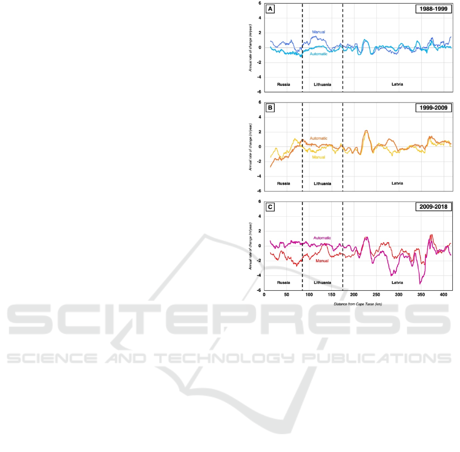
4.2.2 Spatial Accuracy Analysis of the

Results

The analysis of the coastline extraction methods'

spatial accuracy allows for observing the spatial

divergence of the results (Figure 5). For each decade,

we calculated a moving average trend chart with the

annual variations of the two coastline extraction

methods. To smooth the results and show significant

fluctuations, the average threshold is defined on 200

values.

For the period 1988-1999, the largest differences

between the annual shoreline variations of the two

methods of shoreline extraction are located on the

coast of the Curonian Spit. In the rest of the study

area, both charts follow the same evolution trends

(Figure 5).

For the period 1999-2009, the differences in

annual shoreline variation between the coastline

extraction methods are small with the exception of the

Sambian and Curonian coasts. The manual method of

extraction models a retreat of the Lithuanian part of

the Curonian Spit, while the automatic method of

extraction shows an accretion for example (Figure 5).

There is also a clear divergence in the modelling

of shoreline evolution in the proximity of the Latvian

port of Pavilosta (270 km), with an accretion of the

coast for the automatic method and a significant

retreat for the manual method.

The differences in annual variation between the

extraction methods are the most significant in the

period 2009-2018. The spatial modelling is less

accurate because of the cloud cover, which implies

potentially larger margins of error.

For Russia and the Lithuanian mainland, the

results of the manual method show a clear erosion (–

1.29 m/year and –1.16 m/year), whereas the results of

the automatic method indicate overall stability (0.24

m/year and 0.03 m/year). A very strong retreat of the

Latvian coast can be observed using the automatic

coastline (–1.31 m/year). The erosion rate is more

modest for the calculations performed with the manual

coastlines (–0.62 m/year). The trend remains identical

for both spatial modelling methods (Figure 5).

Figure 5: Averaged trend charts of annual inter-period

variations for automatic and manual methods of extraction

of the coastline for the periods (a) 1988-1999, (b) 1999-

Cyclical dynamics are also observed over time

and regardless of the extraction method. These

variations are most often characterised by rapid peaks

of variation which correspond in their location to the

presence of port areas: Sventoji (170 km), Liepaja (225

km), Pavilosta (270 km), and Ventspils (335 km).

5 DISCUSSIONS

5.1 Natural and Anthropogenic Factors

Explaining the Evolution of the

Coastline

In this research, we highlighted an alternation

between eroding and accreting areas during the period

1988-1999 regardless of the extraction method used

(Figure 5). These coastal dynamics are representative

of the spatial redistribution of sediments conditioned

by the inflow and outflow of longshore drift along the

southeast coast of the Baltic Sea.

The Evolution of the South-Eastern Baltic Sea Coastline Between 1988 and 2018 by Remote Sensing

During the periods 1999-2009 and 2009-2018,

this alternation is disturbed either in favour of more

intense erosion (manual method) or changes in pre-

existing spatial dynamics (automatic method).

The rise in sea level and the increase in extreme

storm events are "natural" processes that can explain

the current evolution of the coastline. They are

responsible for the weakening of the foredunes which

protects against erosion. A large part of the coastline

is vulnerable because it is formed by sandy beaches.

In addition, there is a limited human intervention for

coastal protection in these same areas. Coastal

management consists mainly of beach nourishment,

dune ridge reinforcement and natural fences to fix

vegetation in the dune and capture sand. Many

protected areas have also the objective of protecting

the natural coastal heritage (Gulbinskas et al., 2009;

Nitavska and Zigmunde, 2013; Pranzini, and

Williams, 2013; Spiriajevas, 2014). A weakening of

dune activity can impact sediment supply

(Armaitienė et al., 2007).

This evolution could also reflect the more

sensitive anthropogenic pressures and degradations

on the coast. They manifest themselves in the form of

disturbances to sediment supply and stocks.

Recreational activities are the cause of a

weakening of the dunes when tourists walk off the

signposted paths and damage the dune ridge for

example (Žilinskas, 2008; Pranzini et Williams,

2013). Greater deterioration is observed in areas of

high residential development with houses built

behind the dunes to take advantage of the sea view.

The sedimentary stocks are seriously altered by

sand and gravel extraction activities, which are used

in particular to extend the ports or for construction

activities (Pranzini and Williams, 2013; Žilinskas et

al., 2020).

Changes in coastal dynamics can also be

explained by a disruption of the natural forces that

control the evolution of the coast. The most relevant

examples are ports (Figure 6) where coastal defence

structures (groins, dykes) capture part of the sediment

transport through longshore drift (Bagdanavičiūtė et

al., 2012; Jarmalavičius et al., 2012; Pranzini and

Williams, 2013). Sand captures in these structures

generally cause local erosion and accretion

downstream and upstream respectively. These

structures are also found along the coast of the

Sambian Peninsula (Karmanov et al., 2018).

Figure 6: Evolution of the coastline between 1988 and 2018

in the ports of (a) Liepaja and (b) Ventspils, Latvia.

5.2 Critical Analysis of the

Methodology

5.2.1 Time-Processing

This research provided an opportunity to compare

two remote-sensing coastline extraction methods.

The automatic method represents a significant time

processing advantage over the manual method in

terms of the digitalisation process. This ‘time benefit’

GISTAM 2023 - 9th International Conference on Geographical Information Systems Theory, Applications and Management

increases with the size of the area studied due to the

automation of the processing chain.

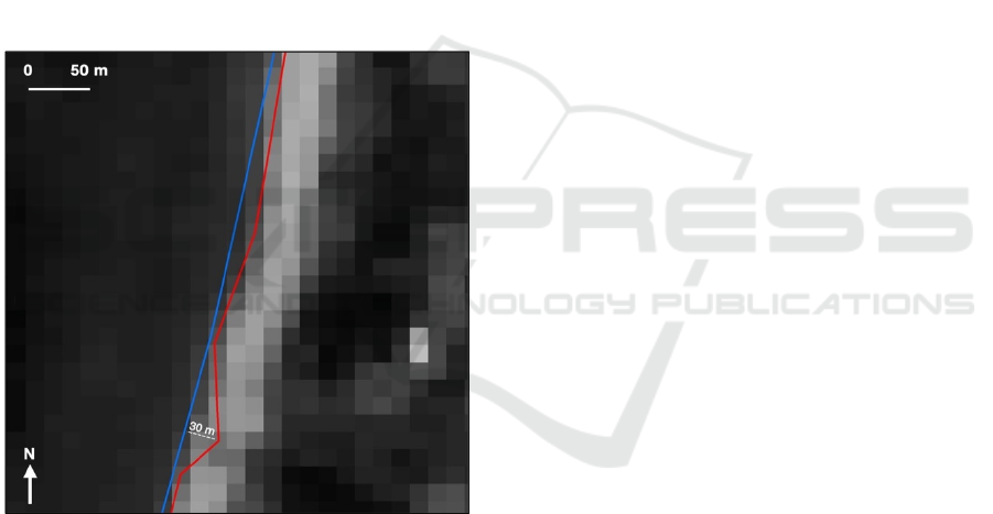
5.2.2 Accuracy of the Shoreline Recognition

The extraction of the coastline with the automatic

method is not directly associated with terrain criteria

such as topography, presence of vegetation, sand

humidity, etc. It depends primarily on the spectral

calibration of the bands, the spectral range covered,

and the spatial resolution. Some limitations of the

automatic coastline extraction method can be

observed. For example, for a given date with an area

overlapping between two satellite scenes, the

coastline will be interpreted differently (Figure 7).

The delimitation by the manual method is more

related to ‘scientific’ criteria but requires knowledge

and understanding of satellite images, which is also

indirectly dependent on the quality of the image

processing.

Figure 7: Two coastlines interpreted differently according

to the automatic extraction method for the same date, the

same area but with two superimposed satellite images.

5.2.3 Comparison of the Results

The automatic method presents robust results

between the calculations of the multi-year coastal

variations with and without weighting by the most

reliable data.

Over the period 1988-2018, the results obtained

with the manual method, weighted by the most reliable

data, are similar to those obtained with the automatic

method, independently of the weighting or not.

The results analysed by decades, in particular for

the periods 1999-2009 and 2009-2018 show

significant differences between the manual and

automatic approaches. The calculations by decade do

not use the margin of error given for each coastline.

This could explain the differences in the results

between the two methods compared to the multi-

annual calculations made between 1988 and 2018

with the margins of error.

The largest variations are mostly located on wide

beaches (up to 100m wide). The relationship between

spatial resolution and beach width is questionable.

Finally, if we compare the results obtained with

studies carried out on the Russian coast between 2007

and 2017 (Karmanov et al., 2018) or on the

Lithuanian coast between 1947/1955-2010

(Bagdanavičiutė et al., 2012), the results of the

automatic method are systematically the closest

(differences less than 1 m).

6 CONCLUSIONS

In recent decades, coastal erosion has emerged as an

important environmental issue for public authorities

in the south-east Baltic Sea countries.

However, measuring the evolution of the

coastline with Landsat 4-5 TM and Landsat 8 OLI

satellite images between 1988 and 2018 have allowed

us to determine a relative stability with an annual

variation rate of -0.21 m/year.

Nevertheless, the annual rates of change by

decade indicate other trends. During the period 1988-

1999, there is an alternation between eroding and

accreting areas, representative of a redistribution of

sediments by the littoral drift. Calculations for the

periods 1999-2009 and 2009-2018 seem to show a

disruption of this cyclical evolution in favour of more

intense erosion or changing spatial dynamics of

coastal evolution.

New factors of natural origin (rise in sea level,

reduction in ice periods, etc.) or anthropogenic origin

(degradation of dunes, coastal protection structures,

etc.) could cause these changes.

This research also compared two methods of

coastline extraction: manual, by photointerpretation

and automatic, by MNF transformation and Laplacian

enhancement filter of the Landsat multispectral

bands. The automatic method demonstrated its

advantages in terms of processing time and

robustness in terms of results.

Nevertheless, we would like to point out that the

differences between the two methods over the long

term (1988-2018) with calculations including a

margin of error are insignificant. Further

The Evolution of the South-Eastern Baltic Sea Coastline Between 1988 and 2018 by Remote Sensing

developments of this research could consist in using

satellite images with a better spatial resolution such

as Sentinel 2 MSI. However, the relevance of using

the automatic method for the extraction of the

coastline could be questioned by a less complete

spectral resolution than on Landsat satellite images.

Finally, our research could be completed by

multi-source data (aerial photos, field data, historical

maps) to control the results of the satellite image

analysis. Nevertheless, these data are not

systematically available, of satisfactory quality and

standardised for our study area, in the time period

analysed.

ACKNOWLEDGEMENTS

This research is supported by the CNES AICMEE

TOSCA programme (Apport de l’Imagerie

satellitaire Multi-Capteurs pour répondre aux Enjeux

Environnementaux et sociétaux des socio-systèmes

urbains).

REFERENCES

Armaitienė, A., Boldyrev, V.L., Povilanskas, R.,

Taminskas, J. (2007). Integrated shoreline management

and tourism development on the cross-border World

Heritage Site: A case study from the Curonian spit

(Lithuania/Russia). The Journal of Coastal

Conversation, 11(1), 13-22.

Bagdanavičiutė, I, Kelpšaitė, L. Daunys, D. (2012).

Assessment of shoreline changes along the Lithuanian

Baltic Sea coast during the period 1947-2010. Baltica

25(2), 171-184.

Bird, E. (2010). Encyclopedia of the world’s coastal

landforms. Springer Sciences & Business Media.

Bitinas, A., Žaromskis, R., Gulbinskas, S., Damusytė, A.,

Žilinskas, G., Jarmalavičius, D. (2005). The results of

integrated investigations of the Lithuanian coast of the

Baltic Sea: geology, geomorphology, dynamics, and

human impact. Geological Quaterly, 49(4), 355-362.

Björkqvist, J.V., Pärt, S., Alari, V., Rikka, S., Lindgren, E.,

Tuomi, L. (2021). Swell hindcast statistics for the Baltic

Sea. Ocean Sciences, 17(6), 1815-1829.

Brunina, L., Rivza, P., Konstantinova, E. (2011). Coastal

Spatial Planning Problems in Latvia. Journal of Coastal

Research, 1224-1227.

Burnashov, E. (2011). Current coastal dynamics in the

Kaliningrad region, based on annual monitoring

surveys. Issues of modern science and practice.

Vernadsky University. IV Vernadsky, (2), 10-17.

Eaglet, V. (1999). Environmental problems of the Baltic

Sea and the Kaliningrad region.

European Space Agency Climate Change Initiative, Land

Cover project. (2017). 300 m Annual Global Land

Cover Time Series from 1992 to 2015. Retrieved from

https://www.esa-landcover-cci.org/?q=noe/175.

Faye, I., Giraudet, E., Gourmelon, F., Hénaff, A. (2011).

Cartographie normalisée de l’évolution du trait de côte.

Mappemonde, 104(4). Retrieved from https://map

pemonde-archive.mgm.fr/num32/articles/art11404.htlm.

Fedorov, G.M., Kunetsova, T., Razumovkii, V.M. (2017).

How the Proximity of the Sea Affects Development of

Economy and the Settlement in Kaliningrad Oblast.

Regional Research of Russia, 7(4), 352-362.

Fisher, R., Perkins, S., Walker, A., Wolfart, E. (2000).

Hypermedia Image Processing Reference (HIPR2).

Retrieved from https://homepages.inf.ed.ac.uk/rbf/

HIPR2/log.htm.

Gadal, S., Gloaguen, T. (2021). Environmental issues in the

coastal regions of the south-eastern Baltic Sea: A

sensitive natural environment in the face of increasing

anthropic pressures. Baltica, 34(2), 203-215.

Gulbinskas, S., Suzdalev, S. Mileriene, R. (2009). Coastal

management measures in Lithuanian Baltic coast

(South-Eastern Baltic). Coastal Engineering 2008: (In

5 Volumes), 4042-4052.

Harff, J., Furmańczyk, K., von Storch, H. (2017). Coastline

Changes of the Baltic Sea from South to East. Springer

Cham.

Jakimavičius, D., Kriaučiūnienė, J., Šarauskienė, D. (2018).

Assessment of wave climate and energy resources in the

Baltic Sea nearshore (Lithuanian territorial water).

Oceanologia, 60(2), 207-218.

Jarmalavičius, D., Žilinskas, G., Kulvičienė, G. (2001).

Peculiarities of long-term water level fluctuations on

the Lithuanian Coast. Acta Zoological Lituanica, 11(2),

132-140.

Jarmalavičius, D., Žilinskas, G., Kulvičienė, G. (2012).

Impact of Klaipeda port jetties reconstruction on

adjacent seacoast dynamics. Journal of Environmental

Engineering and Landscape Management, 20(3), 240-

247.

Karmanov, K. Burnashov, E., Chubarenko, B. (2018)

Contemporary Dynamics of the Sea Shore of

Kaliningrad Oblast. Archives of Hydro-Engineering

and Environmental Mechanics, 143-159.

Łabuz, T.A. (2015). Environmental impacts — coastal

erosion and coastline changes. In: Second Assessment

of Climate Change for the Baltic Sea Basin, 381-396.

Springer, Cham.

Lépy, E. (2012). Baltic Sea ice and environmental and

societal implications from the comparative analysis of

the Bay of Bothnia and the Gulf of Riga. Fennia-

International Journal of Geography, 190(2), 90-101.

Libeesh, N., Naseer, K., Mahmoud, K., Sayyed, M.,

Arivazhagan, S., Alqahtani, M., El Sayed, Y.,

Khandaker, M. (2022). Applicability of the

multispectral remote sensing on determining the natural

rock complexes distribution and their evaluability on

the radiation protection applications. Radiation Physics

and Chemistry, 193.

Nitaska, N., Zigmunde, D. (2013) The impact of

legislatives rules and economic development on the

coastal landscape in Latvia. CIVIL ENGINEERING’13,

259.

GISTAM 2023 - 9th International Conference on Geographical Information Systems Theory, Applications and Management

Olenina, I., Olenin, S. (2002). Environmental Problems of

the South-Eastern Baltic Coast and the Curonian

Lagoon. In: Schernewski, G., Schiewer, U. Baltic Coast

Ecosystems. Central and Eastern European

Development Studies, 149-156. Springer, Berlin.

Pranzini, E., Williams, A. (2013). Coastal Erosion and

Protection in Europe. Routledge.

Safaval, A., Kheirkhah, Z., Neshaei, S., Ejlali, F. (2018).

Morphological changes in the southern coasts of the

Capsian Sea using remote sensing and GIS. Caspian

Journal of Environmental Sciences, 16(3), 271-285.

Soomere, T. (2013). Extending the observed Baltic Sea

wave climate back to the 1940s. Journal of Coastal

Research, 65, 1969-1974.

Spiriajevas, E. (2014). Hindrances and suggestion for

sustainable development of Lithuanian Coastal Strip

(Zone). Regional Formation and Development Studies,

6(1), 125-136.

Syarif, A., Kumara, S. (2018). The effect of minimum noise

fraction on multispectral imagery data for vegetation

canopy density modelling. Geoplanning: Journal of

Geomatics and Planning, 5(2), 251-258.

Thieler, E., Himmelstoss, E., Zichichi, J., Ergul, A. (2018).

Digital Shoreline Analysis System (DSAS) version 5.0.

– An ArcGIS extension for calculating shoreline

change. US Geological Survey.

Vermillion, S.C., Sader, S.A. (1999). Use of the minimum

noise fraction (MNF) transform to analyze airbone

visible/infrared imaging spectrometer (AVIRIS) data of

northern forest types. In AVRIRIS workshop, 7.

Vogt, J., Soille, P., De Jager, A. Rimaviciute, E., Mehl, W.,

Foisneau, S., Bodis, K., Dusart, J., Paracchini, M.L.,

Haastrup, P., Bamps, C. (2007). A pan-European river

and catchment database. Report EUR 22920.

Weisse, R., Dailidienė, I., Hünicke, B., Kahma, K.,

Madsen, K., Omstedt, A., Parnell, K., Schöne, T.,

Sommere, T., Zhang, W., Zorita, E. (2021). Sea level

dynamics and coastal erosion in the Baltic Sea region.

Earth System Dynamics. 12, 871–898.

Zanaga, D., Van De Kerchove, R., Daems, D., De

Keersmaecker, W., Brockmann, C., Kirches, G.,

Wevers, J., Cartus, O., Santoro, M., Fritz, S., Lesiv, M.,

Herold, M., Tsendbazar, N.E., Xu, P., Ramoino, F.,

Arino, O. (2022). ESA WorldCover 10 m 2021 v200.

Žilinskas, G. (2008). Distinguishing priority sectors for the

Lithuanian Baltic Sea coastal management. Baltica,

21(1-2), 85-94.

Žilinskas, G., Janušaitė, R., Jarmalavičius, D., Pupienis, D.

(2020). The impact of Klaipeda Port entrance channel

dredging on the dynamics of coastal zone, Lithuania.

Oceanologia, 62(4), 489-500.

The Evolution of the South-Eastern Baltic Sea Coastline Between 1988 and 2018 by Remote Sensing