Comprehensive Differentiation of Partitional Clusterings

Lars Sch

utz

1,2 a

, Korinna Bade

1 b

and Andreas N

urnberger

2 c

Department of Computer Science and Languages, Anhalt University of Applied Sciences, K

othen (Anhalt), Germany

Faculty of Computer Science, Otto von Guericke University Magdeburg, Magdeburg, Germany

Keywords:

Clustering Difference Model, Cluster Comparison, Applications in Planning and Decision Processes.

Abstract:

Clustering data is a major task in machine learning. From a user’s perspective, one particular challenge in this

area is the differentiation of at least two clusterings. This is especially true when users have to compare clus-

terings down to the smallest detail. In this paper, we focus on the identiﬁcation of such clustering differences.

We propose a novel clustering difference model for partitional clusterings. It allows the computational detec-

tion of differences between partitional clusterings by keeping a full description of changes in input, output,

and model parameters. For this purpose, we also introduce a complete and ﬂexible partitional clustering rep-

resentation. Both the partitional clustering representation and the partitional clustering difference model can

be applied to unsupervised and semi-supervised learning scenarios. Finally, we demonstrate the usefulness of

the proposed partitional clustering difference model through its application to real-world use cases in planning

and decision processes of the e-participation domain.

1 INTRODUCTION

Machine learning algorithms and models have been

successfully applied to numerous domains of our lives

for many years. However, one major challenge is that

machine learning algorithms and models are not al-

ways easy to interpret. In this context, interpretability

describes the extent to which a person can understand

the cause of a decision (Miller, 2019) or how much

a person can reliably predict the result of a machine

learning model (Kim et al., 2016). We frequently have

to explain the decisions or recommendations that have

been generated by machine learning algorithms and

models. We should at least be curious about this, es-

pecially when these algorithms and models have a sig-

niﬁcant impact on our environment and personal lives.

It is immediately noticeable that humans play a cen-

tral role when it comes to utilizing machine learning

algorithms and models.

Clustering data sets is a very common task in ma-

chine learning which we will focus on in this paper.

The general clustering objective is to partition a set

of data instances into a (pre-deﬁned) number of clus-

ters or partitions. Data instances can either belong

to only one cluster (hard clustering) or to multiple

https://orcid.org/0000-0003-3303-6619

https://orcid.org/0000-0001-9139-8947

https://orcid.org/0000-0003-4311-0624

clusters at the same time (soft clustering). In this

work, we speciﬁcally focus on partitional clustering

in unsupervised and semi-supervised learning scenar-

ios. In unsupervised clustering, there is no further

information about the relationship between the data

instances, and there is no prior assignment to a clus-

ter for any of the data instances at hand. Well known

clustering algorithms are k-means (Lloyd, 1982; Mac-

Queen, 1967), k-medoids (Kaufman and Rousseeuw,

1987; Schubert and Rousseeuw, 2019), and fuzzy c-

means (Bezdek, 1981). In contrast, there is some

supervision available in semi-supervised clustering.

For instance, this supervision can describe the re-

lationship between parts of the data instances. In

this regard, pairwise constraints are commonly used

to model whether two data instances must belong

to the same cluster (must-link) or to two distinct

clusters instead (cannot-link) (Wagstaff et al., 2001).

Exemplary semi-supervised clustering algorithms are

instance-based pairwise-constrained k-means (Basu

et al., 2004) and metric-based pairwise-constrained k-

means (Bilenko et al., 2004).

Different clustering algorithms and algorithm pa-

rameter settings lead to different clusterings of the

same data set. How can we distinguish between these

clusterings? The comprehensive differentiation of

clusterings is challenging. We generally have difﬁ-

culties to track changes or differences (Simons and

Schütz, L., Bade, K. and Nürnberger, A.

Comprehensive Differentiation of Partitional Clusterings.

DOI: 10.5220/0011762000003467

In Proceedings of the 25th International Conference on Enterprise Information Systems (ICEIS 2023) - Volume 2, pages 243-255

ISBN: 978-989-758-648-4; ISSN: 2184-4992

 2023 by SCITEPRESS – Science and Technology Publications, Lda. Under CC license (CC BY-NC-ND 4.0)

243

Rensink, 2005). For example, while it might be easy

for us to differentiate the number of computed clus-

ters per clustering, it might be more difﬁcult for us

to identify modiﬁed data instances as well as data in-

stances that have different cluster assignments. We

may even think there are no differences at all simply

because we have not noticed them. We follow the idea

that changes should be communicated in order to en-

sure a sound understanding of the involved machine

learning models (Kulesza et al., 2012; Kulesza et al.,

2013; Kulesza et al., 2015). This also applies to the

clustering differences. But these kind of differences

must ﬁrst be detected before they can be communi-

cated properly. Enabling this detection in a ﬂawless

and detailed way is our major motivation.

The detection of clustering differences becomes

even more crucial in interactive or human-in-the-loop

clustering (Coden et al., 2017). In such clustering sce-

narios, the user guides the clustering algorithms and

models by interacting with the computer systems and

software applications that encompass them. This al-

lows the integration of user knowledge, e. g., the user

can correct automatically computed assignments of

data instances to clusters. In turn, such user inter-

action can trigger changes in the involved clustering

during the clustering process. The clustering might

even change several times if we consider frequent user

interaction. These clustering differences matter. They

do not only allow the user to compare clusterings for

evaluating their overall quality. They also enable the

user to understand the consequences of her interac-

tions. So in the end, it is possible that the user will

be confused during the interactive clustering process

when the differences or changes are not communi-

cated properly. However, it must ﬁrst be possible to

detect these differences.

In this paper, our main contribution is the intro-

duction of a novel partitional clustering difference

model (Section 4). It allows the computational de-

tection of differences between partitional clusterings.

This paper is the ﬁrst fundamental work following

this speciﬁc approach. The novel partitional clus-

tering difference model is based on a ﬂexible parti-

tional clustering representation which we also present

in this paper (Section 3). Additionally, we demon-

strate the applicability and practicability of the model

by the means of exemplary but still prominent real-

world use cases in planning and decision processes

of the e-participation domain (Section 5). Further-

more, we present related work (Section 2), we con-

clude our research presented in this paper (Section 6),

and we point to major directions for future work in

this area (Section 7).

2 RELATED WORK

Generally, our research is in line with the recommen-

dations of the ethics guidelines for trustworthy arti-

ﬁcial intelligence published by the High-level Expert

Group on Artiﬁcial Intelligence that was set up by the

European Commission (High-Level Expert Group on

AI, 2019). In their list of four ethical principles and

seven key requirements for realizing trustworthy arti-

ﬁcial intelligence, they emphasize human agency, hu-

man oversight, and explicability of machine learning

algorithms and models. This clearly correlates to our

motivation. However, they do not provide concrete

methods and implementation options for any machine

learning algorithm or model. The encouraging point

is that the necessity of methods for interpretable ma-

chine learning and explainable artiﬁcial intelligence

has long been recognized (Lipton, 2018; Abdul et al.,

2018). However, this broad ﬁeld is still considered

to be very challenging so that related research activ-

ities continue to increase for years (Doshi-Velez and

Kim, 2017). In particular, a lot of research activities

in this area are being carried out for supervised learn-

ing scenarios, especially concerning the understand-

ing of artiﬁcial deep neural networks, while efforts

in the unsupervised and semi-supervised learning sce-

narios seem to be less frequent.

We focus on the differences between clusterings.

We want to make clustering changes transparent. The

work that examines the general comparison or dif-

ferentiation of clusterings is clearly closely related

research. In this regard, there are many measures

that compare different clusterings (Wagner and Wag-

ner, 2007). Commonly, these measures are classiﬁed

into at least three groups: pair-counting measures,

e. g., the Rand index (Rand, 1971), measures based

on overlapping sets, e. g., the “Meil

a-Heckerman-

Measure” (Meil

a and Heckerman, 2001), and infor-

mation theoretic measures (Vinh et al., 2010), e. g.,

the variation of information (Meil

a, 2003; Meil

2005; Meil

a, 2007). These measures are sometimes

used to evaluate the quality of clusterings in com-

parison to ground truth labels if these are available,

and these measures are also used to check how simi-

lar or dissimilar clusterings are. Unfortunately, these

measures do not consider the differences between at

least two clusterings in relation to the data instances

and their cluster assignments on a lower level, i. e.,

changes to cluster assignments of individual data in-

stances cannot be determined by relying only on these

measures. Instead, these measures allow a high-level

comparison of clusterings. The similarity or dissimi-

larity of clusterings is only represented by a number

which is the numerical value of the speciﬁc measure

ICEIS 2023 - 25th International Conference on Enterprise Information Systems

244

used. It remains unclear where the differences be-

tween the clusterings exactly are. We, however, con-

sider a full description of differences between cluster-

ings on the lowest level.

Other closely related research that addresses mul-

tiple different clusterings are meta clustering and con-

sensus clustering methods. For example, the meta

clustering algorithm (Caruana et al., 2006) generates

various reasonable and qualitatively different cluster-

ings on a base level. These are then presented to a

user on a meta level, e. g., by clustering similar clus-

terings. In the end, this user is free to select the most

appropriate (meta) clustering. Again, it remains un-

clear where the differences between the clusterings

exactly are. This applies to the clusterings on the base

and meta levels. The user also needs to determine

the differences independently. Consensus clustering,

e. g., cluster ensemble methods (Strehl and Ghosh,

2003), typically tries to ﬁnd the maximum agree-

ment between multiple clusterings in order to gener-

ate one single clustering that is supposed to be bet-

ter than the individual ones, i. e., such methods focus

on how much information is shared. This approach

also does not detect the exact clustering differences

on the lowest level. A detailed differentiation of clus-

terings from a user’s perspective is not possible with

this approach. We consider a different path by provid-

ing a formal model description of the plain difference

between clusterings. We see this description as the

foundation for communicating changes to a user. To

the best of our knowledge, there is no prior work fol-

lowing this speciﬁc idea.

3 PARTITIONAL CLUSTERING

REPRESENTATION

In order to be able to differentiate partitional cluster-

ings, we need to deﬁne a partitional clustering repre-

sentation ﬁrst. For this purpose, we have the follow-

ing requirements:

1. Completeness: The partitional clustering repre-

sentation shall be as complete and comprehensive

as possible so that the difference between two par-

titional clusterings can also be determined in de-

tail as much as possible. This requirement is about

not losing any information that might later be use-

ful to the user.

2. Flexibility: The partitional clustering representa-

tion should be separated from the partitional clus-

tering algorithm as much as possible so that it is

beneﬁcial for a wider range of clustering applica-

tions, i. e., the partitional clustering representation

needs to be ﬂexible to some extent.

First, we consider a matrix D ∈ R

N×M

that conforms

to the complete parent data set available for learning

the partitional clustering. The N rows and M columns

of D represent the data instances and data features re-

spectively. D

i,∗

denotes the i-th data instance of D,

1 ≤ i ≤ N, and D

∗, j

denotes the j-th data feature of D,

1 ≤ j ≤ M. Consequently, the row and column in-

dices of D act as the data instance and data feature

identiﬁers. We assume that there is exactly one par-

ent data set. Furthermore, we allow the selection

of a n × m submatrix X of D for learning the parti-

tional clustering so that only speciﬁc data instances

and data features can be used, n ≤ N, m ≤ M. Then

we ﬁnally consider the partitional clustering represen-

tation (r, c, C, W, Y, p):

• A vector r ∈ N

representing the selected data in-

stance identiﬁers. It describes the mapping from

data instance identiﬁers to row indices of X. The

i-th vector entry r

is the data instance identiﬁer

of X

i,∗

, 1 ≤ i ≤ n. The row index i of X does

not necessarily have to match the data instance

identiﬁer. For example, X

1,∗

could actually repre-

sent the eleventh data instance of the parent data

set D, i. e. X

1,∗

= D

11,∗

, instead of the ﬁrst one,

i. e. X

1,∗

6= D

1,∗

• A vector c ∈ N

representing the selected data

feature identiﬁers. It acts as the mapping from

data feature identiﬁers to column indices of X.

The j-th vector entry c

is the data feature iden-

tiﬁer of X

∗, j

, 1 ≤ j ≤ m. The column indices of X

do not necessarily have to match the data feature

identiﬁers.

• A matrix C ∈ {−1, 0, 1}

n×n

conforming to the

pairwise constraints between the data instances.

The entry C

i, j

denotes a pairwise constraint be-

tween the i-th data instance and the j-th data in-

stance, 1 ≤ i ≤ n, 1 ≤ j ≤ n. We consider three

distinct values for the entries: C

i, j

= −1 indicates

a cannot-link constraint, C

i, j

= 1 indicates a must-

link constraint, and there is no pairwise constraint

between i and j when C

i, j

= 0.

• A matrix W ∈ {w ∈ R | w ≥ 0}

n×n

denoting the

weights of the pairwise constraints. The en-

try W

i, j

controls the importance of the related

pairwise constraint C

i, j

, 1 ≤ i ≤ n, 1 ≤ j ≤ n. For

example, the larger the entry, the greater the im-

portance.

• A matrix Y ∈ {y ∈ R | 0 ≤ y ≤ 1}

n×k

correspond-

ing to the cluster assignments of all data instances.

The number of clusters is denoted by k ∈ N. The

entry Y

i, j

represents the cluster assignment of the

Comprehensive Differentiation of Partitional Clusterings

245

data instance i to the cluster j, 1 ≤ i ≤ n, 1 ≤ j ≤ k.

It holds

∑

j=1

i, j

= 1, ∀i. The column indices

of Y act as the cluster identiﬁers.

• A tuple p containing the partitional clustering pa-

rameters. The number and structure of the tu-

ple entries depend on the applied clustering algo-

rithm. For example, p could contain the mean

vectors and covariance matrices of multivariate

Gaussian mixture components.

We categorize the aforementioned components into

three groups: r, c, C, and W belong to the input pa-

rameters, Y belongs to the output parameters, and p

belongs to the model parameters. These groups pro-

vide a complete and comprehensive representation of

the clustering (requirement 1).

We consider our partitional clustering represen-

tation as a general and ﬂexible union of different

ways to formalize unsupervised and semi-supervised

partitional clustering representations (requirement 2).

First, if the semi-supervised learning scenario is not

of interest, we can ignore the related components C

and W. This depends on the learning scenario and the

available expert knowledge or supervision. Second,

the chosen matrix structure of Y allows us to consider

soft clustering, i. e., Y

i, j

∈ [0, 1], as well as hard clus-

tering, i. e., Y

i, j

∈ {0, 1}. Third, the model parame-

ters p further increase the degree of ﬂexibility. The-

orem 3.1 describes the (storage) space complexity of

the partitional clustering representation.

Theorem 3.1. Let pc = (r, c, C, W, Y, p) be a par-

titional clustering according to the deﬁnition of the

partitional clustering representation, let f

and f

denote the (storage) space of pc and p respectively,

and let O(·) denote asymptotic notation. Then f

O(max(n

, f

)) holds true.

Proof. Since pc is composed of r, c, C, W, Y, and p,

the (storage) space f

equals the sum f

+ f

of the individual (storage) spaces. So

we have f

= n+m+nn+nn+nk+ f

. Considering

that n  k in clustering tasks, we ﬁnally have f

O(max(n

, f

)).

We emphasize that we consider exactly one par-

ent data set for a comparison of different partitional

clusterings. If we were to consider multiple parent

data sets from different instance and feature spaces

instead, the differentiation of the related partitional

clusterings would be pointless. This means that a

change to D will be reﬂected to all involved partitional

clusterings. And ﬁnally, please note that possibly a

lot of entries of C and W are zero. Hence, C and W

can be represented as sparse matrices instead. Go-

ing further, the redundant constraints that follow the

symmetric property C

i, j

= C

j,i

can also be removed,

i. e., C and W could be represented as upper or lower

triangular matrices.

4 PARTITIONAL CLUSTERING

DIFFERENCE MODEL

We now propose the novel partitional clustering

difference model. It is represented by the tu-

ple (r

, c

, C

, W

, Y

, p

). This tuple representation

is similar to the partitional clustering representation

introduced in the previous section. The compo-

nents r

, c

, C

, W

, Y

, and p

semantically relate to

their counterparts r, c, C, W, Y, and p of the partitional

clustering representation. However, each component

now describes a difference, i. e., given two partitional

clusterings pc

= (r

, c

, C

, W

, Y

, p

) and pc

, c

, C

, W

, Y

, p

), r

describes the difference be-

tween r

and r

, and c

describes the difference be-

tween c

and c

etc. These component-wise differ-

ences on the lowest level lead to a full description of

the overall difference. This approach allows us to de-

tect changes to the input parameters, the output pa-

rameters, and the model parameters.

Each component of the partitional clustering

difference model is represented by the ordered

triple (cm, add, rem). It entails the following three

vectors: common entries or modiﬁed entries cm,

added entries add, and removed entries rem. The vec-

tor add represents the entries that have been added to

the involved component of pc

, and the vector rem

represents the entries that have been removed from

the involved component of pc

. In contrast, there are

subtle differences in the interpretation of cm. Refer-

ring to r

, the vector cm represents the common data

instance identiﬁers existing in both r

and r

. The

same applies to c

and the common data feature iden-

tiﬁers. But when referring to C

and W

, the vec-

tor cm represents the exact values of the differences

between the modiﬁed constraints and weights respec-

tively. The same applies to Y

, i. e., the vector cm

represents the exact values of the differences between

the modiﬁed cluster assignments of the data instances.

In summary, by considering a component difference

as the ordered triple (cm, add, rem), we can carefully

ﬁnd out which exact difference or type of change

exists. On the contrary, this approach may already

seem complex or rather laborious because, for only

one partitional clustering difference, we already have

to deal with six ordered triples (one ordered triple

for each partitional clustering difference component),

and each ordered triple entry is represented by a vec-

tor which further increases the complexity. However,

ICEIS 2023 - 25th International Conference on Enterprise Information Systems

246

in this regard, we just aim for a complete, compre-

hensive, and fundamental model of partitional clus-

tering differences at ﬁrst. It is not about the direct or

immediate interpretation of the partitional clustering

difference model from a user’s perspective.

We now brieﬂy describe the computation of the

individual component differences. Following our def-

inition of the partitional clustering representation, we

need to consider differences between vectors (r and c),

matrices (C, W, and Y), and tuples (p). The com-

putation of each component difference results in an

ordered triple of the form (cm, add, rem) as we de-

scribed before. Referring to the difference r

between

the two vectors r

and r

of two partitional cluster-

ings, cm then contains the entries that r

and r

have

in common, add holds the entries that are contained

in r

but not in r

, and rem holds the entries that are

contained in r

but not in r

. The same applies to the

computation of c

. The computation of the matrix dif-

ferences C

, W

, and Y

is more sophisticated because

it has to take the data instance identiﬁers, data feature

identiﬁers, and cluster identiﬁers into account. We

provide a novel, detailed algorithm for the computa-

tion of these special kind of matrix differences in ﬁg-

ure 1.

This algorithm returns the ordered

triple (cm, add, rem) that represents the differ-

ence between two matrices M

and M

. Finally,

considering the tuple difference p

, the differences

are computed for each component of the tuple

analogously. We assume that the type and semantics

of the model parameters p are ﬁxed.

We want to point out that it might be beneﬁcial to

consider a sparse vector representation for the vec-

tor cm that entails either common or modiﬁed val-

ues, especially if there are only subtle differences be-

tween the involved partitional clusterings. This would

have a positive effect on the (storage) space of the

partitional clustering difference model. The (storage)

space complexity is described by Theorem 4.1. Ad-

ditionally, if there is no difference between the com-

ponents of the partitional clusterings at all, the vec-

tors cm, add, and rem are empty vectors which we de-

note by ∅.

Theorem 4.1. Let pcd = d(pc

, pc

) =

, c

, C

, W

, Y

, p

) be the partitional cluster-

ing difference between the partitional cluster-

ings pc

= (r

, c

, C

, W

, Y

, p

) and pc

, c

, C

, W

, Y

, p

) according to the deﬁnition of

the partitional clustering difference model, let f

pcd

and f

denote the (storage) space of pcd and p

respectively, and let O(·) denote asymptotic notation.

Then it follows f

pcd

= O (max(n

+ n

, f

)).

Proof. Since pcd is composed of r

, c

, C

, W

, Y

Algorithm: Difference between two matrices of dif-

ferent sizes

Input:

1) Matrices M

∈ R

s×t

and M

∈ R

u×v

2) Vectors r

∈ N

, c

∈ N

, r

∈ N

, and c

∈ N

that represent the row and column identiﬁers

of M

and M

Output: Matrix difference M

between M

and M

Remark:

1) set(v) returns a set with the elements of vector v

2) replace(a, b) replaces all a

of vector a with a

’s

index in vector b

3) vec(M) returns the matrix M as a vector in row-

major order

4) M[i; j] denotes the submatrix of the matrix M

formed from the r rows given by the row indices

vector i = [i

, i

, . . . , i

] and the c columns given

by the column indices vector j = [ j

, j

, . . . , j

]

5) sparse(v) returns a sparse vector representation

of the (dense) vector v

Method:

1) Compute common row and column identiﬁers

1.1) Row identiﬁers r := set(r

) ∩ set(r

)

1.2) Column identiﬁers c := set(c

) ∩ set(c

)

2) Compute common row and column indices

2.1) Row indices i

of M

:= replace(r, r

)

2.2) Column indices j

of M

:= replace(c, c

)

2.3) Row indices i

of M

:= replace(r, r

)

2.4) Column indices j

of M

:= replace(c, c

)

3) Compute modiﬁed, added, and removed entries

3.1) mod := sparse(vec(M

] − M

]))

(use of sparse is optional)

3.2) add := vec(entries of M

exclud-

ing M

])

3.3) rem := vec(entries of M

exclud-

ing M

])

4) Return M

= (mod, add, rem)

Figure 1: Matrix difference algorithm for computing C

, W

and Y

of the partitional clustering difference model.

and p

, the (storage) space f

pcd

equals the sum f

+ f

of the individual (storage)

spaces. We have f

= n

+ n

− |φ(r

) ∩ φ(r

)|, f

+ m

− |φ(r

) ∩ φ(r

)|, f

= f

= n

+ n

−

|φ(r

) ∩ φ(r

)|, f

= n

+ n

− |φ(r

) ∩ φ(r

)|,

φ(v) returns a set containing the unique elements of

the vector v. Considering that n

 k

and n

 k

in clustering tasks, this leads to f

pcd

= O(max(n

, f

)).

We provide a detailed example for determining

a partitional clustering difference between two parti-

tional clusterings in Example 4.1 to better illustrate

the previous descriptions.

Comprehensive Differentiation of Partitional Clusterings

247

Example 4.1. Let D denote the parent data set for

learning partitional clusterings as stated in (1).

D =







1 1 1

1 2 2

2 1 3

2 2 4







(1)

Furthermore, consider the two speciﬁc partitional

clusterings pc

and pc

that used D as stated in (2)

and (3) respectively. Figure 2 depicts pc

and pc

= ([1, 2, 3], [1, 2], 0

3×3

, 0

3×3





1 0

0 1





, (2)) (2)

= ([1, 2, 4], [1, 2], 0

3×3

, 0

3×3





1 0

0 1





, (2)) (3)

0 1 2

∗,1

∗,2

0 1 2

∗,1

∗,2

Figure 2: Two exemplary partitional clusterings pc

(left)

and pc

(right) with two clusters each (indicated by marker

shape and color).

Both partitional clusterings have only one model pa-

rameter k = 2 that explicitly speciﬁes the number of

clusters. Then the difference of pc

and pc

yields

the partitional clustering difference pcd = d(pc

, pc

) =

, c

, C

, W

, Y

, p

). The difference of the data instance

identiﬁers r

is stated in (4), and the difference of the data

feature identiﬁers c

is stated in (5).

= d(r

, r

) = ([1, 2], [4], [3]) (4)

= d(c

, c

) = ([1, 2], ∅, ∅) (5)

These equations demonstrate that the data instance with

identiﬁer 4 has been used to learn pc

(but not pc

), the data

instance with identiﬁer 3 has been used to learn pc

(but

not pc

), the ﬁrst two data instances of D have been used

to learn both pc

and pc

, and that both partitional clus-

terings have been learned using the ﬁrst two data features

only. The difference C

is then stated in (6).

= d(C

, C

, r

, c

, r

, c

)

= (0, 0, 0, 0], [0, 0, 0, 0, 0], [0, 0, 0, 0, 0])

(6)

No values have been modiﬁed, but there are added and re-

moved values because of the difference r

. The difference W

is computed analogously. Finally, the differences Y

and p

are stated in (7) and (8) respectively.

= d(Y

, Y

, r

, c

, r

, c

) = ([0, 0, 0, 0], [0, 1], [0, 1]) (7)

= d(p

, p

) = (0) (8)

We explicitly point out that the computation of

the partitional clustering difference model will dif-

ferentiate clusterings even if only the cluster identi-

ﬁers have been swapped between partitional cluster-

ings. In this case, all clusters could still contain the

same data instances as before. Although this is for-

mally a difference, such a difference might not be of

interest. Then this could be corrected by incorporat-

ing model parameters like the cluster centers to check

for the equality of the clusters, or a mapping from

cluster identiﬁers to column indices of the cluster as-

signments matrix Y could be added to the partitional

clustering representation as we did with the data in-

stance and data feature identiﬁers. But we will not

focus on this speciﬁc aspect in this paper any further.

5 USE CASES

In this section, we apply the proposed partitional clus-

tering difference model. By this means, we demon-

strate the usefulness and potential of this novel model.

We also demonstrate its beneﬁts in comparison to the

partitional clustering representation. Overall, our ob-

jective is to motivate for the necessity of the parti-

tional clustering difference model in speciﬁc situa-

tions. At the same time, we emphasize that this is

fundamental work conducted more on a conceptual

level.

We concentrate on exemplary but still prominent

real-world use cases in the area of planning and

decision processes (Pahl-Weber and Henckel, 2008;

Blotevogel et al., 2014). These processes play a cru-

cial role in the e-participation domain where people

are allowed to voice their opinions and ideas in dif-

ferent areas such as landscape planning or city bud-

geting (Briassoulis, 1997). Overall, such planning

and decision processes can last several days, weeks,

months, or even years. During that time, special

phases exist where people are allowed to participate.

In the end, participants write and submit contributions

that should be assessed by public administrations.

The public administration workers need to make de-

cisions, e. g., they aggregate ideas for a new building

project, or they accept or reject general complaints.

We consider the following scenario for the use

cases: A public administration worker needs to an-

alyze a data set of 1590 contributions submitted by

citizens. These contributions consist of textual data

(content of the contribution), time-oriented data (cre-

ation time), and spatial data (longitude and latitude

representing the contribution’s reference point). Ta-

ble 1 shows an exemplary contribution. The data set

originates from a real past participation phase of a

ICEIS 2023 - 25th International Conference on Enterprise Information Systems

248

Table 1: An exemplary contribution.

Content Timestamp Longitude Latitude

The cobblestones are in a very poor condition. They cause

a high level of noise pollution. Even the current speed limit

does not help here, especially since this is ignored by many

drivers.

2021-05-23T09:25 13.4577 52.5128

planning and decision process. The contributions re-

port city noise sources. The city intends to take ac-

tion against the most common noise sources. There-

fore, the public administration worker’s objective is

to ﬁnd partitions of similar contributions. Generally,

the motivation behind this is that similar contribu-

tions can be assessed and dealt with in a fairly sim-

ilar way which would reduce the amount of work for

the public administration worker. Such a partitioning

helps to aggregate the different topics or complaints

submitted by the citizens. The public administra-

tion worker is assisted by a machine learning system

that is able to cluster the contributions by incorpo-

rating the k-means algorithm and the instance-based

pairwise-constrained k-means algorithm (only in the

fourth use case). The public administration worker

could cluster the contributions one by one and com-

pare the own results to the clustering proposed by the

machine learning system, or the public administration

worker could explore different clusterings by experi-

menting with parameters of the machine learning sys-

tem. We point out that we consider the k-means al-

gorithm for demonstration purposes only. We could

have used other partitional clustering algorithms such

as k-medoids or k-medians due to our ﬂexible parti-

tional clustering representation.

The proposed partitional clustering difference

model can be used in various situations and for differ-

ent reasons when clustering the contributions. We fo-

cus on the following speciﬁc use cases: (1) Debug the

clustering algorithm, (2) Change the number of clus-

ters, (3) Detect changes in the data set, and (4) Create

constraints. These reﬂect common interactions (Bae

et al., 2020). The machine learning system would

compute the difference between clusterings.

5.1 Debug the Clustering Algorithm

This use case is about the traceability of each itera-

tion of the clustering algorithm, e. g., when the ini-

tial clustering of the contributions is learned, or every

time the public administration worker wants the ma-

chine learning system to re-compute the clustering.

Sometimes, such a profound understanding is neces-

sary, especially if the computed clustering is adopted

by the public administration worker (with or without

further user-made adjustments) in order to make ma-

jor and possibly impactful decisions as we mentioned

in the introduction of this paper. Additionally, pub-

lic administration workers are laypersons in the ﬁeld

of machine learning. At least a brief understanding

of how the machine learning system works in practice

can be useful when it comes to trusting and accepting

the computed clusterings.

In this use case, the public administration worker

can examine the clustering at each iteration of the

learning process which refers to analyzing a sequence

of partitional clusterings. Our proposed partitional

clustering representation can be used for this purpose

to gain comprehensive and complete insights. We ac-

knowledge that this procedure is generally not a novel

approach. In fact, such a method is already used for

teaching or educational purposes at least. But never-

theless, there is still a downside that we emphasize:

the public administration worker would have to com-

pare the partitional clusterings on her own. Then, for

example, it might be difﬁcult to grasp the exact differ-

ences between the initial and ﬁnal clusterings. On the

contrary, the partitional clustering difference model

allows a new perspective. The public administration

worker can apply the partitional clustering difference

model to ﬁnd out how the clustering of the contribu-

tions changes either step by step or by examining the

difference between non-sequential partitional cluster-

ings.

Figure 3 depicts partitional clusterings of the ﬁrst,

second last, and last iterations of the clustering algo-

rithm

and the partitional clustering differences be-

tween them. While the sequence of partitional clus-

terings allows a general overview of the clustering for

every iteration, the sequence of partitional clustering

differences explicitly shows how many contributions

We used the textual content of the contributions. First,

we removed non-alphanumeric characters from the textual

content. Then we tokenized the textual content, converted

it to lower case, and, ﬁnally, we stemmed the results us-

ing the Porter stemmer algorithm. Second, we used the re-

sulting tokens to create a term-document matrix with term

frequency–inverse document frequency (TF–IDF) weights.

Third, we performed latent semantic indexing on this ma-

trix to derive ten concepts. We randomly picked three initial

cluster centers from the data set of contributions.

Comprehensive Differentiation of Partitional Clusterings

249

−80 −60 −40 −20 0 20 40 60

−50

∗,1

∗,2

−80 −60 −40 −20 0 20 40 60

−50

∗,1

∗,2

−80 −60 −40 −20 0 20 40 60

−50

∗,1

∗,2

−60 −40 −20 0 20 40 60

−50

∗,1

∗,2

−60 −40 −20 0 20 40 60

−50

∗,1

∗,2

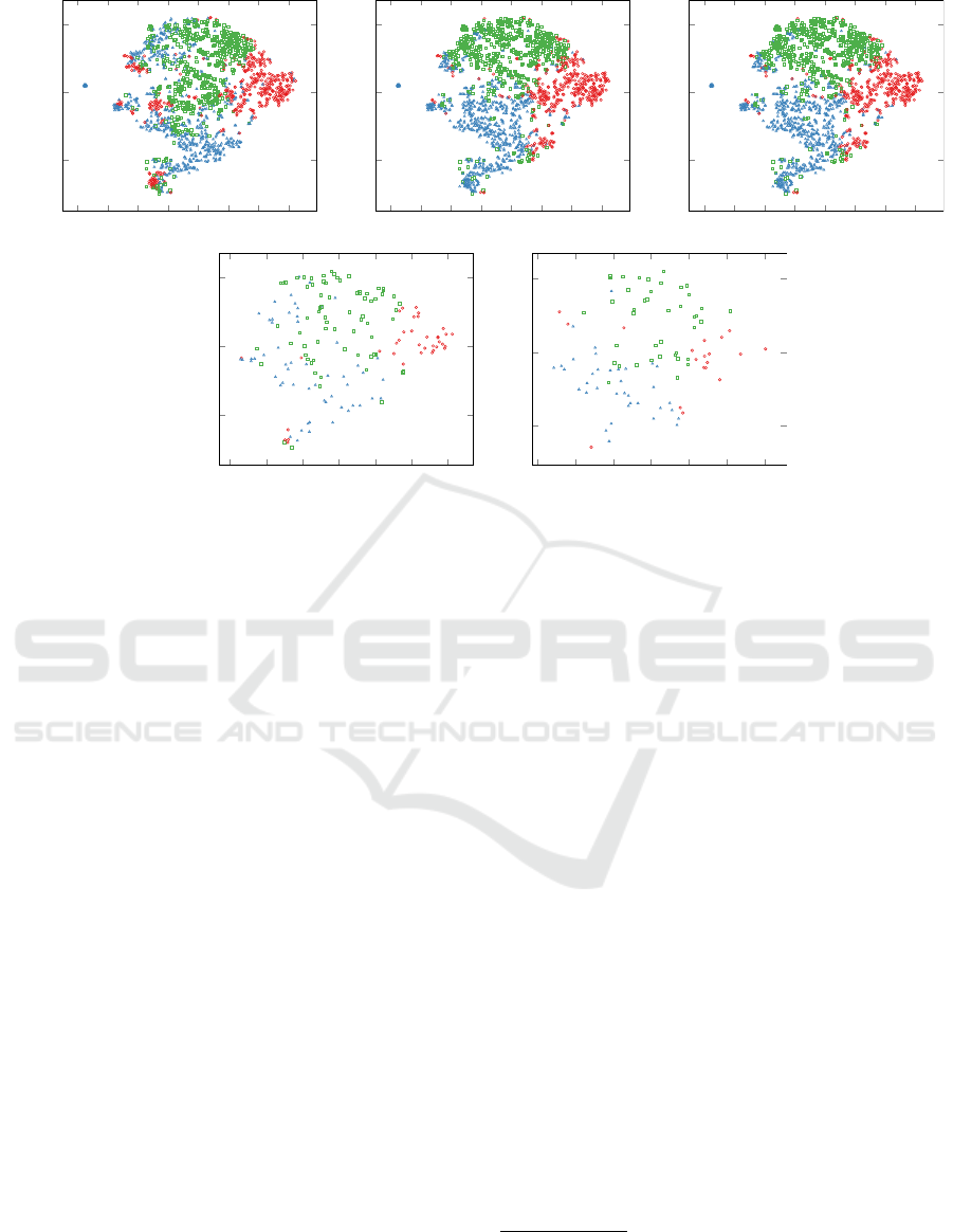
Figure 3: Partitional clusterings (top, from left to right) and related partitional clustering differences (bottom, from left to

right) between these partitional clusterings with three clusters (indicated by marker shape and color). The term-frequency–

inverse document frequency (TF–IDF) vector representations of the contributions’ contents used for clustering have been

reduced to two dimensions using a t-distributed stochastic neighbor embedding (t-SNE) for demonstration purposes only.

are assigned to different clusters in comparison to the

previous iteration. Of course, it is still difﬁcult to

specify the exact quantity of affected contributions

by only relying on this speciﬁc visualization. This

clearly depends on the overall number of contribu-

tions. But from iteration to iteration, there should be

fewer differences visible according to how the cluster-

ing algorithm works. Figure 3 conﬁrms this. Thus,

the public administration worker can get more insight

into how the clustering algorithm generally works by

applying the partitional clustering difference model.

Please note again that we provide only sample visu-

alizations for demonstration purposes. The visual en-

coding of the partitional clustering difference model

is not the focus of this paper. However, this does not

change the fact that this model contains all the infor-

mation needed to communicate the exact differences

between each iteration. The model could also be the

foundation for deriving further metrics such as the ex-

act quantity of changes.

5.2 Change the Number of Clusters

During the clustering task, the public administration

worker might increase or decrease the number of clus-

ters in order to compare appropriate clusterings of the

contributions. This can be seen as an optimization

step of a clustering model parameter from an expert’s

perspective. But this can also be seen as some kind

of experimentation with algorithm or user interface

settings from a layperson’s perspective. The public

administration worker might alternately increment or

decrement the number of clusters just to get an idea

of the effects on the clustering result computed by

the machine learning system. Either way, this spe-

ciﬁc user interaction will most likely affect the cluster

assignments of some contributions, i. e., some contri-

butions keep their previous cluster assignments, and

others get new cluster assignments. It is important

for the public administration worker to notice these

differences, especially when the public administration

worker tries to build a mental model of the underlying

concept that represents the clustering. But it can be

challenging to ﬁrst grasp and then evaluate this con-

cept if the clustering changes without communicating

the differences.

Figure 4 shows a small sample of 51 contributions

for demonstration purposes only. It illustrates how the

cluster assignments of these contributions differ from

each other when the public administration worker de-

creases the number of clusters used by the clustering

algorithm

from k = 3 to k = 2. The simple juxtaposi-

Again, we focused on the textual content, and we ap-

plied the same preprocessing steps as in the ﬁrst use case.

We used k-means++ seeding for sequentially choosing the

initial cluster centers.

ICEIS 2023 - 25th International Conference on Enterprise Information Systems

250

100 105 110 115 120 125 130 135 140 145 150

i,∗

100 105 110 115 120 125 130 135 140 145 150

i,∗

100 105 110 115 120 125 130 135 140 145 150

i,∗

Figure 4: Two partitional clustering assignments (top and

middle) of the contributions from 100 to 150 (from left

to right) to a maximum of three clusters (differentiated by

marker shape and color) and the difference (bottom).

tion of both partitional clustering assignments (before

and after the change) together with the sorting of the

contributions allows the public administration worker

to search for differences. The public administration

worker should be able to identify the differences by

scanning through the whole list of contributions and

their assignments. This is not a novel idea, and such

a visual juxtaposition can be easily generated even

without our introduced partitional clustering repre-

sentation. But there are still issues left. The pub-

lic administration worker can overlook differences, or

the public administration worker may require more

efforts to ﬁnd these. This work is already laborious

for 51 contributions. Generally, this depends at least

on the number of contributions, the number of clus-

ters (before and after the change), and the user’s cog-

nitive abilities. Then this is exactly where the par-

titional clustering difference model assists the pub-

lic administration worker in ﬁnding and analyzing the

differences between the cluster assignments more ef-

ﬁciently. For example, instead of communicating pos-

sibly large lists that contain the previous and current

cluster assignments of the individual contributions to

the public administration worker, only the speciﬁc

contributions that actually changed their assignment

can be presented to the public administration worker.

Then the public administration worker does not have

to search for these differences because they have al-

ready been detected computationally. A condensed

programmatic output of the partitional clustering dif-

ference for this example is shown in Figuere 5. This

output can be the foundation for a new visualization

that communicates the differences.

PCD = (r’, c’, C’, W’, Y’, p’):

r’ = ..., c’ = ...,

C’ = ..., W’ = ...,

p’ = ...,

Y’ = (mod, add, rem)

= ([(107, 2->3), ..., (134, 2->1)],

[], [])

Figure 5: Condensed programmatic output of the partitional

clustering difference between the two clusterings shown in

Figure 4. The output partially lists the affected contribu-

tions and their new cluster assignments, e. g., the contribu-

tion 107 now belongs to cluster 3.

5.3 Detect Changes in the Data Set

The contributions submitted to the public administra-

tion can change in planning and decision processes of

the e-participation domain. There are various reasons

for this circumstance. For example, the data set of

contributions might not always be complete when the

public administration worker starts the clustering pro-

cess, which means that new contributions can arrive

later. Public administrations sometimes start to an-

alyze the contributions even though the participation

phase is still running. This can happen when the data

set of contributions is large and the assignments of

parts of the contributions must be controlled manually

by the public administration. So in order to cope with

the data set volume, the public administration worker

may want to start early with clustering the contribu-

tions available at this speciﬁc point in time. This

problem becomes more prominent when the user-

driven clustering process takes multiple hours or even

days with possible breaks in between while new con-

tributions can still be submitted by the participants.

Another example is the deletion or editing of some

contributions after the initial submission. This can

be done by the owners or submitters of the contri-

butions. For example, participants sometimes correct

the location the contribution points to, assuming that

such information is collected at all, or the participants

sometimes edit the content after the initial submis-

sion. Such a change should be taken into account be-

cause the contribution could suddenly portray a com-

pletely different meaning or complaint. Furthermore,

the machine learning system could learn a completely

different clustering by taking the added, removed, and

modiﬁed contributions into account. This new clus-

tering and the reasons for the re-computation, i. e.,

the changes to the contributions, should then be com-

municated to the public administration worker. The

public administration worker should be able to differ-

entiate the proposed two clusterings before and after

Comprehensive Differentiation of Partitional Clusterings

251

the changes to the data set of contributions.

Another perspective and motivation for the parti-

tional clustering difference model is that the changes

to the contributions cannot be controlled by the public

administration worker who wants to cluster the data

set. This missing control means that some kind of

detection and notiﬁcation could be useful to inform

the public administration worker about the change or

difference in the data set because it might affect the

overall clustering result when known contributions

are suddenly missing, have been changed, or when

new contributions reveal new relationships or ideas.

While the public administration worker could pos-

sibly just ignore deleted contributions in the current

clustering, added contributions must still be assessed

and put into the correct cluster by the public adminis-

tration worker.

Figure 6 illustrates a sample of 100 contributions

from our real-world data set at two different points in

time during the participation phase. It immediately

becomes clear that it is challenging to identify all dif-

ferences. This is especially true when there are no

further hints to suggest what to look for. This prob-

lem is not restricted to this exemplary visualization

that focuses on the spatial data of the contributions.

We could also arrange the contributions side by side

while focusing on the textual content (before and af-

ter the changes), and the identiﬁcation of differences

would probably be even more challenging. But by us-

ing the partitional clustering difference model instead,

the public administration worker can easily identify

the differences between the data sets because it tracks

the exact changes to the data instances and data fea-

tures used to actually learn a partitional clustering. In

this use case, it detects added, removed, and modiﬁed

contributions. So overall, the number of contributions

changed because there are more additions of contri-

butions than removals. One edit occurred. Again, the

public administration worker can retrieve this data set

difference by analyzing the partitional clustering dif-

ference. Such a simple quantiﬁcation can still be done

without our model. However, the public administra-

tion worker is also able to retrieve which exact con-

tributions changed, have been removed, or are com-

pletely new.

5.4 Create Constraints

The automatically computed assignments of contri-

butions to clusters are not always correct so that the

public administration worker wants to integrate some

corrections. In this use case, the public administra-

tion worker adds a few pairwise constraints to make

some corrections to the partitional clustering com-

puted by the clustering algorithm, i. e., some contri-

butions shall belong to the same cluster if possible be-

cause they represent a similar concern that the cluster-

ing algorithm did not detect. Based on this new infor-

mation, the machine learning system can re-compute

the clustering with a potentially better quality. In

turn, this new clustering can be presented to the pub-

lic administration worker. But the addition of pair-

wise constraints not only inﬂuences the clustering as-

signments. The clustering algorithm, in this use case

the instance-based pairwise-constrained k-means al-

gorithm, also has to re-compute the transitive closure

of the pairwise constraints every time a pairwise con-

straint is added, i. e., the clustering algorithm derives

new pairwise constraints, or it needs to remove exist-

ing ones. This is also true when the public adminis-

tration worker deletes some pairwise constraints be-

tween the contributions. Even if the public adminis-

tration worker explicitly adds only one pairwise con-

straint, other pairwise constraints can also be affected.

It is possible that multiple new must-link constraints

are added implicitly, although the public administra-

tion worker has explicitly added only one must-link

constraint. This is not only a difference triggered by

the public administration worker but also a difference

triggered by the clustering algorithm. Such a distinc-

tion can be important. These effects might be clear

to an expert user with background knowledge in ma-

chine learning. But a layperson like the public ad-

ministration worker might not know about the prop-

erties of pairwise constraints. However, the effects on

the relations between contributions should be made

clear, especially if it can affect the clustering result.

The public administration worker should investigate

implicitly added constraints in order to improve the

understanding of the relations between the involved

contributions. Furthermore, the larger the number of

contributions the more challenging it is for the public

administration worker to manually keep track of the

implicitly changed pairwise constraints.

Table 2 lists ﬁve must-link constraints that the

public administration worker added explicitly. Based

on these, three more must-link constraints have been

added implicitly by the clustering algorithm. The par-

titional clustering difference model can keep track of

these differences. The public administration worker

can then inspect the new proposed relations between

the contributions by considering the implicitly as well

as the explicitly added pairwise constraints.

ICEIS 2023 - 25th International Conference on Enterprise Information Systems

252

13.1 13.2 13.3 13.4 13.5 13.6 13.7

52.4

52.5

52.6

longitude

latitude

13.1 13.2 13.3 13.4 13.5 13.6 13.7

52.4

52.5

52.6

longitude

latitude

13.1 13.2 13.3 13.4 13.5 13.6 13.7

52.4

52.5

52.6

longitude

latitude

Figure 6: The data set of contributions with a sample of 100 contributions at two different points in time during the partici-

pation phase (left and middle), and the difference between these data sets (right). It shows added contributions (red, circular

marker), removed contributions (blue, triangular marker), and one modiﬁed contribution (green, rectangular marker; the ﬁlled

marker style represents the contribution before the modiﬁcation).

Table 2: Explicitly and implicitly added must-link con-

straints between the contributions x

and x

Constraints

Explicit Implicit

1 1 34 65 98 1 2 2

2 34 66 67 99 66 34 66

6 CONCLUSION

Our work focused on revealing the differences be-

tween partitional clusterings. We introduced a novel

partitional clustering difference model for the differ-

entiation of two partitional clusterings. It is equally

suitable for unsupervised and semi-supervised clus-

tering because it can store information about differ-

ences between pairwise constraints that typically rep-

resent some form of supervision. In general, this par-

titional clustering difference model keeps track of all

changes to the input, output and model parameters of

the involved partitional clusterings. Consequently, it

does not only track differences between clustering as-

signments but also between input parameters like the

data instances and data features used to learn the par-

titional clusterings. The exact clustering differences

become transparent.

The partitional clustering difference model is

valuable for clustering comparison tasks. A user can-

not always be sure that no clustering differences ac-

tually exist just because none were found by the user.

The novel partitional clustering difference model de-

tects all differences without error and with no human

efforts instead. We demonstrated the potential of the

partitional clustering difference model by applying it

to different prominent real-world use cases in the e-

participation domain. Nonetheless, future work is still

needed.

7 FUTURE WORK

There is signiﬁcant potential for future work due to

the novelty of the proposed partitional clustering dif-

ference model and its potential. The related ideas

involve different research areas. First, it should be

investigated how the partitional clustering difference

model can be efﬁciently communicated to a user.

We provided some visualizations in this paper but

for demonstration purposes only. We need to decide

which information should be shown to and which in-

formation should be hidden from the user. Thus, the

research and application of proper visualization tech-

niques for the differentiation of partitional clusterings

is an important part of possible future work. In this

regard, general visualization techniques like juxtapo-

sition, explicit encoding, and superposition (Gleicher

et al., 2011) should be investigated further. Espe-

cially ways to visually encode at least parts of a parti-

tional clustering difference should be studied and de-

veloped. Second, we would like to examine how the

model can be combined with the standard evaluation

measures mentioned in Section 2. This concerns both

the application of existing standard evaluation mea-

sures and the formulation of new measures in order

to express the magnitude of the differences. Third,

we would like to conduct user studies with layper-

sons to evaluate the appropriateness of the partitional

clustering difference model at least in the described

use cases. For this purpose, intelligent user interfaces

need to be researched and developed that integrate the

partitional clustering difference model in the cluster-

ing process. Overall, this is an interdisciplinary topic.

Comprehensive Differentiation of Partitional Clusterings

253

REFERENCES

Abdul, A., Vermeulen, J., Wang, D., Lim, B. Y., and

Kankanhalli, M. (2018). Trends and trajectories for

explainable, accountable and intelligible systems: An

HCI research agenda. In Proceedings of the 2018 CHI

Conference on Human Factors in Computing Systems,

pages 582:1–582:18, New York, NY, USA. ACM.

Bae, J., Helldin, T., Riveiro, M., Nowaczyk, S., Bouguelia,

M.-R., and Falkman, G. (2020). Interactive clustering:

A comprehensive review. ACM Computing Surveys,

53(1):1:1–1:39.

Basu, S., Banerjee, A., and Mooney, R. J. (2004). Active

semi-supervision for pairwise constrained clustering.

In Proceedings of the 2004 SIAM International Con-

ference on Data Mining, pages 333–344, Lake Buena

Vista, Florida, USA. Society for Industrial and Ap-

plied Mathematics.

Bezdek, J. C. (1981). Pattern Recognition with Fuzzy Ob-

jective Function Algorithms. Advanced Applications

in Pattern Recognition. Springer US, New York, NY,

USA.

Bilenko, M., Basu, S., and Mooney, R. J. (2004). Integrat-

ing constraints and metric learning in semi-supervised

clustering. In 21st International Conference on Ma-

chine Learning, page 11, Banff, Alberta, Canada.

ACM Press.

Blotevogel, H. H., Danielzyk, R., and M

unter, A. (2014).

Spatial planning in germany. In Spatial planning sys-

tems and practices in Europe. Routledge Taylor &

Francis Group, London, UK and New York, NY, USA.

Briassoulis, H. (1997). How the others plan: Exploring

the shape and forms of informal planning. Journal

of Planning Education and Research, 17(2):105–117.

Caruana, R., Elhawary, M., Nguyen, N., and Smith, C.

(2006). Meta clustering. In 6th International Con-

ference on Data Mining, pages 107–118, Hong Kong,

China. IEEE.

Coden, A., Danilevsky, M., Gruhl, D., Kato, L., and Na-

garajan, M. (2017). A method to accelerate human in

the loop clustering. In Proceedings of the 2017 SIAM

International Conference on Data Mining, Proceed-

ings, pages 237–245, Houston, Texas, USA. Society

for Industrial and Applied Mathematics.

Doshi-Velez, F. and Kim, B. (2017). Towards a rigorous

science of interpretable machine learning.

Gleicher, M., Albers, D., Walker, R., Jusuﬁ, I., Hansen,

C. D., and Roberts, J. C. (2011). Visual comparison

for information visualization. Information Visualiza-

tion, 10(4):289–309.

High-Level Expert Group on AI (2019). Ethics guidelines

for trustworthy AI. Report, European Commission,

Brussels.

Kaufman, L. and Rousseeuw, P. J. (1987). Clustering by

means of medoids. In Statistical Data Analysis Based

on the L1-Norm and Related Methods, pages 405–

416. Elsevier Science, Amsterdam, North-Holland;

New York, NY., USA.

Kim, B., Khanna, R., and Koyejo, O. O. (2016). Exam-

ples are not enough, learn to criticize! Criticism for

interpretability. In Advances in Neural Information

Processing Systems 29, pages 2280–2288. Curran As-

sociates, Inc., Barcelona, Spain.

Kulesza, T., Burnett, M., Wong, W.-K., and Stumpf, S.

(2015). Principles of explanatory debugging to per-

sonalize interactive machine learning. In Proceed-

ings of the 20th International Conference on Intelli-

gent User Interfaces, pages 126–137, Atlanta, Geor-

gia, USA. ACM.

Kulesza, T., Stumpf, S., Burnett, M., and Kwan, I. (2012).

Tell me more? the effects of mental model sound-

ness on personalizing an intelligent agent. In Proceed-

ings of the SIGCHI Conference on Human Factors in

Computing Systems, pages 1–10, Austin, Texas, USA.

ACM.

Kulesza, T., Stumpf, S., Burnett, M., Yang, S., Kwan, I.,

and Wong, W.-K. (2013). Too much, too little, or just

right? Ways explanations impact end users’ mental

models. In 2013 IEEE Symposium on Visual Lan-

guages and Human Centric Computing, pages 3–10,

San Jose, CA, USA. IEEE.

Lipton, Z. C. (2018). The mythos of model interpretability:

In machine learning, the concept of interpretability is

both important and slippery. Queue, 16(3):31–57.

Lloyd, S. P. (1982). Least squares quantization in

PCM. IEEE Transactions on Information Theory,

28(2):129–137.

MacQueen, J. (1967). Some methods for classiﬁcation and

analysis of multivariate observations. In Proceed-

ings of the Fifth Berkeley Symposium on Mathemat-

ical Statistics and Probability, Volume 1: Statistics,

pages 281–297, Berkeley, CA, USA. The Regents of

the University of California.

Meil

a, M. (2003). Comparing clusterings by the varia-

tion of information. In Learning Theory and Kernel

Machines, Lecture Notes in Computer Science, pages

173–187, Berlin, Heidelberg. Springer.

Meil

a, M. (2005). Comparing clusterings: An axiomatic

view. In Proceedings of the 22nd International Con-

ference on Machine Learning, pages 577–584, Bonn,

Germany. ACM Press.

Meil

a, M. (2007). Comparing clusterings—an informa-

tion based distance. Journal of Multivariate Analysis,

98(5):873–895.

Meil

a, M. and Heckerman, D. (2001). An experimental

comparison of model-based clustering methods. Ma-

chine Learning, 42(1):9–29.

Miller, T. (2019). Explanation in artiﬁcial intelligence: In-

sights from the social sciences. Artiﬁcial Intelligence,

267:1–38.

Pahl-Weber, E. and Henckel, D., editors (2008). The

planning system and planning terms in Germany.

Academy for Spatial Research and Planning, Hanover,

DE.

Rand, W. M. (1971). Objective criteria for the evaluation of

clustering methods. Journal of the American Statisti-

cal Association, 66(336):846–850.

Schubert, E. and Rousseeuw, P. J. (2019). Faster k-

medoids clustering: Improving the PAM, CLARA,

and CLARANS algorithms. In Similarity Search and

ICEIS 2023 - 25th International Conference on Enterprise Information Systems

254

Applications, Lecture Notes in Computer Science,

pages 171–187, Cham. Springer International Pub-

lishing.

Simons, D. and Rensink, R. (2005). Change blindness:

Past, present, and future. Trends in cognitive sciences,

9:16–20.

Strehl, A. and Ghosh, J. (2003). Cluster ensembles — a

knowledge reuse framework for combining multiple

partitions. Journal of Machine Learning Research,

3:583–617.

Vinh, N. X., Epps, J., and Bailey, J. (2010). Information the-

oretic measures for clusterings comparison: Variants,

properties, normalization and correction for chance.

Journal of Machine Learning Research, 11:2837–

2854.

Wagner, S. and Wagner, D. (2007). Comparing clusterings

– An overview. Technical report, Karlsruhe.

Wagstaff, K., Cardie, C., Rogers, S., and Schr

odl, S.

(2001). Constrained k-means clustering with back-

ground knowledge. In Proceedings of the Eigh-

teenth International Conference on Machine Learn-

ing, pages 577–584, San Francisco, CA, USA. Mor-

gan Kaufmann Publishers Inc.

Comprehensive Differentiation of Partitional Clusterings

255