Long-Distance Directional Dial-a-Ride Problems

∗

Grzegorz Gutowski

and Grzegorz Herman

Theoretical Computer Science, Faculty of Mathematics and Computer Science, Jagiellonian University, Krak

ow, Poland

Keywords:

Vehicle Routing, Dial-a-Ride Problem, Local Change Algorithm.

Abstract:

We consider vehicle routing problems that occur in practice in the context of long-distance ride-sharing. On

the one hand, the instances of our problems share the helpful property that the passengers travel in roughly

the same geographical direction. On the other, the required cost function has ordering-dependent components.

For two such problems, we provide heuristic algorithms employing a dynamic programming optimization of

a sliding window in appropriate linear orders. In the ﬁrst, exemplary problem, we route a single vehicle. In

the second, we route a ﬂeet of vehicles with a coordinated stopover and exchange of passengers. The size of

the sliding window allows for trade-offs between solution qualities and processing times. Both algorithms are

effective and efﬁcient on data sets representing actual travel requests from Hoper, a commercial ride-sharing

service operated by Teroplan S.A. in Poland.

1 INTRODUCTION

In this paper we describe two algorithms for variants

of vehicle routing problems, which are of practical

importance for a company providing a long-distance

door-to-door ride-sharing service. In this setting, the

vehicles and drivers are provided by the operator,

while each passenger requests to travel from an ar-

bitrary pickup to an arbitrary delivery location. The

requests are primarily long-distance, i.e., the travel

distance between pickup and delivery location is in

the order of hundreds of kilometers. The tickets are

usually sold before the travel date and the operator

optimizes the assignment of vehicles and their routes

when all the passenger requests are known.

There is a vast literature on similar problems like

Capacitated Dial-a-Ride (CDARP), Traveling Sales-

man with Pickup and Delivery (PDTSP), or more

generally Vehicle Routing with Pickup and Deliv-

ery (VRPPD), see (Parragh et al., 2008; Molenbruch

et al., 2017; Ho et al., 2018; Tafreshian et al., 2021;

Ritzinger et al., 2022). All of these problems are ver-

sions of the Traveling Salesman Problem with addi-

tional constraints and all are inherently difﬁcult to

solve optimally. There are numerous practical ap-

https://orcid.org/0000-0003-3313-1237

https://orcid.org/0000-0001-6855-8316

∗

This work has been commissioned by Teroplan S.A.

and partially ﬁnanced by European Union funds (grant

number: RPMP.01.02.01-12-0572/16-01)

proaches to these problems based on integer linear

programming (Ropke et al., 2007; Cordeau, 2006;

Kikuchi, 1984), dynamic programming (Psaraftis,

1980; Psaraftis, 1983; Desrosiers et al., 1984; Bianco

et al., 1994), and local search (Savelsbergh, 1990;

Healy and Moll, 1995; Renaud et al., 2000; Renaud

et al., 2002).

In the particular case of our application, we have

found that the following natural structure occurs in

the problem instances. With passengers spending a

signiﬁcant amount of time on board the vehicle, their

natural expectation is for the travel not to take much

longer than necessary. Choosing a ride-sharing op-

erator, they are implicitly accepting some degree of

detours, but should the route stray too much (subjec-

tively) from the direct one, they might become hesi-

tant to choose the same operator again.

On the one hand, this requirement must be repre-

sented in the modeling and inﬂuence the optimization

target. On the other, it suggests an important business

level constraint: In order to avoid carrying passengers

a signiﬁcant distance in the direction perpendicular or

even completely opposite to the one they requested,

it makes sense to assign them initially to a ﬁxed set

of routes, each based on some travel path with a rel-

atively stable long-term direction and serving pickup

and delivery locations not too far from this path. In

our setting, passengers are informed of theses tenta-

tive routes when buying the ticket.

Henceforth, when solving our routing problems,

Gutowski, G. and Herman, G.

Long-Distance Directional Dial-a-Ride Problems.

DOI: 10.5220/0011763600003479

In Proceedings of the 9th International Conference on Vehicle Technology and Intelligent Transport Systems (VEHITS 2023), pages 187-197

ISBN: 978-989-758-652-1; ISSN: 2184-495X

 2023 by SCITEPRESS – Science and Technology Publications, Lda. Under CC license (CC BY-NC-ND 4.0)

187

we can assume that the instances are directional: all

the passengers in a single instance of a problem travel

roughly in the same geographical direction. This al-

lows us to propose practical solutions which may not

be applicable in general, but turn out to be very effec-

tive and efﬁcient in this particular setting.

Traditionally, the cost function being minimized

in vehicle routing is modeled as the distance in the

graph representing the road network. While the

lengths of individual edges might capture something

more than simply the road distance, such model has

the inherent limitation of being context-insensitive

and does not allow to express the requirement of min-

imizing the detours experienced by individual passen-

gers. In Section 2, we introduce a family of cost func-

tions in which the cost of a segment between succes-

sive vehicle stops might depend on the set of pas-

sengers on board. This captures not only the detour

length, but also other metrics important from the point

of view of passenger experience.

In this paper we present solutions for two prob-

lems with the above properties. In Section 3, we limit

our considerations to routing a single vehicle. This

corresponds to a standard Single Vehicle Capacitated

Dial-a-Ride Problem. For this problem it is possible

to develop algorithms based on the aforementioned

techniques. Still, we present our solution as a gentle

introduction to our method that works well for both

problems. In Section 4 we deal with multiple vehicles

and allow for solutions where passengers can change

their vehicles during a designated time-synchronized

stopover. For this problem we have failed to procure

a working solution based on integer linear program-

ming. The main obstacle for that seems to be the

structure of the selected cost function which is dis-

cussed in detail in Section 2.

Both solutions are based on the local search ap-

proach with the following structure. First, we produce

a heuristic linear ordering of the objects (route points,

or passengers) that is a starting point for the optimiza-

tion process. The ﬁnal solution is then obtained using

dynamic programming that optimizes every consec-

utive segment of a ﬁxed-length in this ordering. We

call this technique peephole optimization, in parallel

to a similar technique employed by compilers for code

optimization. An important feature of this method is

its ﬂexible window size, allowing for a trade-off be-

tween solution quality and processing time. This be-

comes very desirable when the costs of a large num-

ber of instances need to be estimated, with only a few

of them being actually solved. This happens when we

use the single-vehicle algorithm as a sub-procedure in

the multiple-vehicle algorithm.

We provide experimental evaluation of our meth-

ods on real-world data sets provided by Teroplan S.A.,

a commercial ride-sharing operator offering the ser-

vice in Poland. See Figure 1 for the maps of the routes

that were used in the evaluations. As these data sets

include problems with a very limited number of pas-

sengers, we also show that the same algorithms are

capable of handling larger, artiﬁcially constructed, in-

stances.

2 COST FUNCTION

Let us begin by formalizing the optimization criteria.

As mentioned in the Introduction, the typical model

employed in vehicle routing is that of a graph dis-

tance. While elegant in its simplicity and helpful from

the point of view of algorithm design, it is unfortu-

nately too simplistic to capture the priorities occurring

in practical business operations.

The primary customers of a ride-sharing operator

are the passengers. From long-term business perspec-

tive it is thus important to consider not only the op-

erating costs, but also the likelihood of passengers

choosing the same operator in the future.

Based on data gathered by Teroplan S.A., the fol-

lowing quantities inﬂuence the perceived quality of

service:

• detour: by how much the distance (or time) trav-

eled by the passenger exceeds the optimal route

they could have taken not sharing a ride;

• stops: how many times the vehicle stops while the

passenger is on board; and

• leeway: with how many other people the passen-

ger travels.

Quite intuitively, passengers prefer to travel on a di-

rect route, without stops, and on a relatively empty

vehicle. Optimization of these goals is very much

against the optimization of operating costs.

It turns out that all of the above can be expressed

in a model, in which the cost of a route segment be-

tween successive vehicle stops is an afﬁne function of

the road distance, with coefﬁcients determined by the

set of passengers on board. Formally, we let the cost

introduced by the segment s be

:= a

· d

+ b

where P

is the set of passengers on board the vehi-

cle (determining the value of coefﬁcients a

and b

and d

is the distance traveled on segment s.

Let us show how such formulation captures the

above aspects of passenger experience.

VEHITS 2023 - 9th International Conference on Vehicle Technology and Intelligent Transport Systems

188

(a) Single vehicle problem. Data con-

tained requests for 8 of 17 national

routes in Poland gathered for 16 months

(b) Multiple vehicle problem. Data contained requests for an international route

spanning parts of Poland, Germany, Netherlands, and Belgium with stopover

close to Polish-German border gathered for 14 months

Figure 1: Maps of routes used for evaluation of algorithms.

Detour. For each passenger p, let

be the optimal

distance between their requested endpoints. Assume

that the “discomfort” cost of a detour of length d can

be expressed as δ(

) · d for some arbitrary function

δ (this might account for the fact that the same abso-

lute detour might be more acceptable when the opti-

mal route is longer). Letting S

be the set of route

segments on which they have been on board, the de-

tour length experienced by passenger p is

∑

s∈S

−

, and the associated cost equals

∑

s∈S

δ(

) · d

−

δ(

) ·

. The ﬁrst term can be incorporated in the

total cost of all segments by making δ(

) contribute

to a

whenever p ∈ P

, and the second term does not

depend on vehicle routes and thus is irrelevant for the

optimization.

Stops. The number of “unnecessary” stops experi-

enced by passenger p is |S

| − 1. To make each of

them introduce a cost of σ, it is enough to add σ to

whenever p ∈ P

Leeway. The experience of (lack of) leeway hap-

pens over time. Therefore the appropriate cost com-

ponent for each passenger p over the segment s can

be expressed as some constant λ (possibly depen-

dent on the capacity of the vehicle), multiplied by

· (|P

| − 1). Again, this cost can be incorporated

into our model by increasing a

by λ · |P

Overall, all required aspects of the cost can be

modeled by taking

∑

p∈P

δ(

) + λ · |P

and b

:= σ · |P

with the values of δ, σ, and λ calibrated to express the

relative importance of the aspects.

In the practical software implementation of our al-

gorithms there are some more constraints that need to

be considered, like for example a maximal total dis-

tance a vehicle can travel. We have decided not to

discuss them in order to keep the presentation cleaner.

3 SINGLE VEHICLE PROBLEM

In this section we are interested in ﬁnding an optimal

route for a single vehicle. The vehicle has a limited

passenger capacity and goes from some initial loca-

tion to some ﬁnal location. On the way it must serve

a set of passengers, each of whom is to be transported

from their pickup location to their delivery location.

It is worth noting that this problem can be solved

using integer linear programming methods, or even

brute force methods (at least for the instance sizes that

we use to evaluate our method). We present our so-

lution, as it easily scales to larger instances, and the

presentation serves as a gentle introduction to our ap-

proach. In Section 4 we employ the same general ap-

proach to solve a more demanding problem, for which

we didn’t ﬁnd a solution based on standard methods.

Let us begin by specifying the problem more for-

mally. We are given a set X of geographic locations.

These include the pickup and delivery locations re-

quested by the passengers, and initial and ﬁnal loca-

tions of the vehicle. Locations can be represented by

vertices of a strongly connected directed graph mod-

eling the road network. However, as detailed routes

are not really relevant to our solution, we will assume

the graph to be the complete graph on X, with the road

distance between each pair of locations x and y given

as d

x,y

Next, we have a set P of passengers to be trans-

ported, with pickup and delivery locations of a pas-

senger p denoted by p

and p

out

, respectively. Each

location might be requested as a pickup and/or deliv-

Long-Distance Directional Dial-a-Ride Problems

189

ery location by some numbers of passengers. In case

of a point which is simultaneously a pickup and a de-

livery location, it always makes sense to let the pas-

sengers being delivered leave the vehicle before the

ones being picked up board it. Therefore we can fo-

cus on the net occupancy change at each point x ∈ X,

computed as

:= |{p ∈ P : p

= x}| − |{p ∈ P : p

out

= x}|.

The vehicle has a limited passenger capacity c, be-

gins the journey at location x

with no passengers on

board, visits every location in X exactly once, and ﬁn-

ishes at location x

after all passengers have been de-

livered.

Now, a solution to the single vehicle problem is a

linear ordering ≺ on X, satisfying the following va-

lidity constraints:

• the vehicle starts and ends as speciﬁed: ∀x ∈

X : x

≼ x ≼ x

• every pickup location is visited before the corre-

sponding delivery location:

∀p ∈ P : p

≼ p

out

, and

• vehicle capacity is never exceeded: ∀x ∈ X : c ≥

∑

y≼x

Whenever a particular ordering is clear from the con-

text, we might refer to its consecutive locations using

indices: x

≺ x

≺ ... ≺ x

To specify optimization criteria, we need to mea-

sure the cost of a particular solution. The detailed

composition of a practical cost function has been dis-

cussed in Section 2. Here, we only assume it to have

the following general properties:

1. The total cost of the solution can be expressed as

the sum of costs of the route segments between

successively visited locations.

2. The cost of each segment might depend on the

road distance d covered on this segment and on

the set V ⊆ X of locations already visited, but not

on the order in which they are visited. This seg-

ment cost function will be denoted as κ(V,d).

Note that the penalties discussed in Section 2 can be

easily expressed in this way, because the set of visited

locations implies the actual set of passengers on board

the vehicle.

Overall, we wish to optimize

≺

n−1

∑

i=0

κ({x

,... ,x

},d

i+1

over all linear orders ≺ satisfying the validity con-

straints. Note, that while our algorithms can work

with arbitrary κ(V,d), for the purpose of experimen-

tal evaluation we use the simplest possible function

κ(V,d) = d that implies optimization of the total dis-

tance traveled by the vehicle.

Being a generalization of the asymmetric Travel-

ing Salesman Problem, this problem is computation-

ally hard (NPO-hard), even when the cost function

satisﬁes the triangle inequality. The best known ap-

proximation ratio for the problem without additional

constraints is 22 + ε (Traub and Vygen, 2020). Thus,

practical solutions, including the one presented in this

work, employ various heuristics.

As outlined in the Introduction, our approach con-

sists of two phases. First, we construct an initial or-

dering of locations satisfying the validity constraints.

Then, we optimize this solution by considering all its

viable “local” reorderings.

While multiple methods following this general

scheme are known in the literature, none of them take

advantage of the speciﬁc nature of our problem in-

stances, discussed in Section 1. Compared, for ex-

ample, to the classic cut-and-rejoin local search al-

gorithm by Lin (Lin, 1965), our optimization phase

can efﬁciently consider larger reshufﬂings by limiting

them to segments of the initial ordering.

We provide more details on both phases in the fol-

lowing subsections.

3.1 Initial Ordering

Let us begin by constructing the initial ordering of

locations. We will not attempt to make it a cost-wise

approximation of the optimum. Instead, we want it to

be “similar” to the optimum wrt. the indices occupied

by particular locations (we will formalize this notion

near the end of Section 3.2).

To this aim, we exploit the assumption of all pas-

sengers sharing a general direction of travel. For each

passenger p, we construct the vector v

representing

the direction from p

to p

out

. From all v

, we com-

pute the average

direction v which should represent

the general direction of travel. Finally, we assign pri-

orities to the locations, highest priority to x

, lowest

to x

, and decreasing priorities to other locations in

the order of their projection on the average direction

The resulting order given by the priorities might

still violate precedence and capacity constraints.

While the second phase of our approach does not for-

mally require them to be satisﬁed, it only ever consid-

ers orders “similar” to the initial one and thus will fail

to ﬁnd a solution if none of those are valid. This issue

The average might be weighted, with weights depend-

ing non-linearly on the distances between pickup and deliv-

ery locations.

VEHITS 2023 - 9th International Conference on Vehicle Technology and Intelligent Transport Systems

190

is easily ﬁxed by making sure that the order is valid

up front.

To achieve this we use the following procedure.

We construct the order by adding locations at the end

one by one. In each step we consider each loca-

tion which has not yet been added and which, when

added at the end, would not violate any of the con-

straints. Among such locations we select the one with

the highest priority.

The above process is easily implemented in time

O(cn + n logn). While in general it does not guaran-

tee to ﬁnd a valid order even if one exists,

we have

never observed such failure in practice.

Indeed, the

orders produced are usually very close to the “purely

projective”. Important discrepancies show up in areas

of mixed pick-ups and deliveries, in which locations

further down the route might need to be visited earlier

in order to prevent capacity constraint violation.

3.2 Peephole Optimization

Given an initial ordering x

≺ x

≺ .. . ≺ x

of loca-

tions, we can frame the peephole optimization algo-

rithm as dynamic programming.

Fixing a parameter w, called the window length,

and denoting by I the set {0,. . .,n} of location in-

dices, each sub-problem

⟨

k,W, j

⟩

to be solved will be

parameterized by:

• a preﬁx length k ∈ I,

• a window W ⊆ {k + 1, . .. ,k + w} ∩ I, and

• a ﬁnal index j ∈ W ∪ {k}.

The solution to the sub-problem

⟨

k,W, j

⟩

will be the

(locally) optimal order of visiting all the locations that

are either in W , or no later than k-th in ≺, i.e., loca-

tions V

k,W

:= {x

,... ,x

}∪{x

: i ∈W }, with x

com-

ing last. In particular, the whole problem is captured

as the sub-problem

⟨

n,∅,n

⟩

A sub-problem

⟨

k,W, j

⟩

is deemed viable if it sat-

isﬁes the following conditions:

• j = 0 implies W = ∅ (no location can be visited

before x

For an example, consider six passengers

A,B,C, D, E,F and a linear route with six points:

out

= C

= D

out

= E

= F

out

= F

out

. A vehicle with capacity 2 can handle this

route, but not once it has picked up both A and B.

Should such unfortunate case ever occur, one can deal

with it by artiﬁcially duplicating each location so that all

pickup and delivery locations are distinct. This might cause

some geographical locations to be visited more than once,

but guarantees to ﬁnd a valid order, in the worst case serving

the passengers one-by-one.

• p

out

= j implies p

∈ V

k,W

(passengers delivered

at the last location have been picked up earlier),

and

• c ≥

∑

y∈V

k,W

(the set of visited locations meets

capacity constraints).

A sub-problem

⟨

k,W, j

⟩

is called canonical if ei-

ther k = 0 or k + w ∈ W . When neither of these

holds then W ∪ {k} is a correct window for preﬁx

length k −1, V

k,W

k−1,W ∪{k}

, and one could replace

sub-problem

⟨

k,W, j

⟩

by the equivalent sub-problem

⟨

k − 1,W ∪ {k}, j

⟩

. Thus, every non-canonical sub-

problem can be reduced to a canonical one, while

non-viable ones can either be assigned inﬁnite cost

or completely removed from the consideration.

We wish to deﬁne locally optimal solution for

a sub-problem, inductively, as a solution that ex-

tends some locally optimal solution for a smaller

sub-problem by visiting one location more and op-

timizing cost over all such extensions. More for-

mally, locally optimal solution to viable canonical

sub-problem

⟨

k,W, j

⟩

is naturally deﬁned as follows:

• j = 0. The only viable sub-problem here is

⟨

0,∅,0

⟩

, with zero cost.

• j = k > 0. With location x

visited last, the pre-

ﬁx length of the sub-problem covering the re-

maining locations must have been smaller than k.

But then, with k + w ∈ W , such situation cannot

be expressed by our parameterization (its window

would also need to contain k + w, exceeding its

allowed size) and thus will simply not be consid-

ered. We thus return an inﬁnite cost. This is a

place in which our solution might not be globally

optimal.

• j > k, j < k + w. With neither x

, nor x

k+w

vis-

ited last, the preﬁx length of the preceding sub-

problem must be the same. This sub-problem

might thus have been

⟨

k,W \ { j}, j

′

⟩

, for an arbi-

trary (legal) j

′

. We consider all of them, augment

their solutions by the segment from x

′

to x

, and

choose the one with minimal cost.

• j = k + w. This case is similar to the previous

one, but we allow the preﬁx length of the preced-

ing sub-problem to be smaller. This sub-problem

might have been

⟨

′

, j

′

⟩

for an arbitrary (le-

gal) k

′

≤ k, k

′

≥ k − w, j

′

, and W

′

= {k

′

+ 1,k

′

2,... ,k} ∪W \ { j}.

Note how the properties assumed of the cost func-

tion ﬁt nicely into this setting. For each transition

between successive sub-problems, their parameteri-

zations prescribe the set of visited locations and the

endpoints (and thus the road distance) of the corre-

sponding segment, and hence its cost. With the costs

Long-Distance Directional Dial-a-Ride Problems

191

being additive, we only need to remember the cost-

optimal solution to each sub-problem.

Note also, that while viability of

⟨

n,∅,n

⟩

does not

by itself imply the validity of the constructed order,

the algorithm is in fact correct. This is because its re-

sult is obtained from a sequence of solutions to viable

sub-problems with successively larger V

k,W

’s. In such

a sequence, the second and third conditions on via-

bility imply respectively the precedence and capacity

constraints.

The number of sub-problems is Θ(nw2

), leading

to the running time of Θ(nw

). One might even

take w := n, making our algorithm a direct analogue

of the standard dynamic programming solution to the

traveling salesman problem (Bellman, 1962; Held and

Karp, 1962), guaranteed to ﬁnd the global optimum.

This course of action might be viable when solving a

relatively small number of instances with small n.

When the number of instances considered be-

comes large, foregoing global optimality by lowering

the window length might be necessary to obtain prac-

tical running times. Such situations occur naturally

when the passengers are to be split between multiple

vehicles, an example of which will be discussed in

Section 4.

To capture the situations in which our algorithm

behaves optimally, let us formally capture the notion

of “similar” orders:

Deﬁnition 1. A permutation π : I 7→ I is w-local iff

for all indices i, j ∈ I

π(i) − π( j) ≥ w =⇒ i > j.

We can now prove the following:

Proposition 2. For an initial order x

≺ . . . ≺ x

and a w-local permutation π : I 7→ I such that π(≺

) := x

π(0)

,... ,x

π(n)

is a solution (i.e., satisﬁes valid-

ity constraints), peephole optimization of ≺ with win-

dow length w returns a result with cost no worse than

π(≺)

Proof. Let us show that for every r = 0, . ..,n, there

exists a viable sub-problem

⟨

k,W, j

⟩

with j = π(r),

for which V

k,W

= {x

π(0)

,... ,x

π(r)

We proceed by induction on r. For r = 0, we

have π(0) = 0, and sub-problem

⟨

0,∅,0

⟩

satisﬁes the

conditions. Now, assume

⟨

k,W, j

⟩

is a viable sub-

problem with j = π(r) and V

k,W

= {x

π(0)

,... ,x

π(r)

Among different equivalent representations of the

sub-problem, we choose the one, possibly non-

canonical, that maximizes k. For this representation,

we have k + 1 /∈ W.

Let j

′

= π(r + 1). If j

′

= k + 1, then

⟨

k + 1,W,k + 1

⟩

is a viable sub-problem satisfying the

conditions for r + 1. Otherwise, we have that k + 1 =

π(r

′

) for some r

′

> r + 1. The assumption on π being

w-local gives that j

′

= π(r + 1) < π(r

′

) + w ≤ k + w,

and

⟨

k,W ∪ { j

′

}, j

′

⟩

is a viable sub-problem satisfy-

ing conditions for r + 1.

As an immediate consequence we get that when-

ever some globally optimal solution is a w-local per-

mutation of the initial order, our algorithm is optimal.

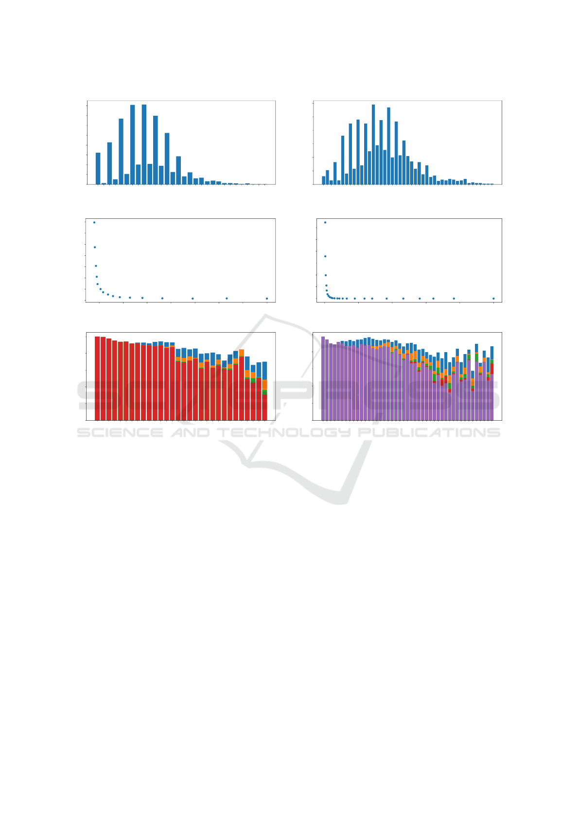
3.3 Evaluation

The experimental data for this problem comes from

the operation of the Hoper ride-sharing service. Pas-

senger requests for 8 different travel routes, out of 17

routes depicted in Figure 1a, have been gathered for

16 months, giving 2970 test cases in total. The ve-

hicles used on these routes were able to accommo-

date 8 passengers. On average, there are 12.2 points

to arrange per test case. Figure 2a shows the dis-

tribution of instance sizes. Observe that the size is

more often an even number (which is to be expected

when pickup and delivery locations are all different).

It seems that at least some of the larger instances were

not really handled by a single vehicle (the best solu-

tions for these cases require to travel more than 2000

kilometers), but we have decided to keep them as they

are.

As mentioned before, for evaluation purposes, we

use κ(V, d) = d as the segment cost, and effectively

we optimize the total distance traveled by the vehi-

cle. The heuristic solution applied to all the test cases

takes 1.6 seconds of CPU time

and ﬁnds routes with

the total distance of 2092549 kilometers. The algo-

rithm with window size set to 16 takes 70 seconds

to compute and gives routes with the total distance

of 1790980 kilometers, saving just above 100 kilo-

meters on average per test case. Solving the largest

test case with 33 locations takes 0.88 seconds to com-

pute. Figure 2c shows the processing time and the to-

tal travel distance for other values of the window size.

Figure 2e shows the quality gain for different sizes of

test cases (measured in the number of locations) for

window sizes 4, 8, 12, and 16.

It is worth noticing that most, but not all, of the

cases in this data set can easily be solved by a brute-

force algorithm that checks all the possible orderings

of the locations. In order to evaluate our solution on

larger instances we have artiﬁcially constructed a new

data set, where each test case is constructed from two

cases corresponding to the same route in the origi-

nal data set by combining the passenger requests and

All computations were performed on a single core of

an Intel Xeon Gold 6154 processor

VEHITS 2023 - 9th International Conference on Vehicle Technology and Intelligent Transport Systems

192

4 5 6 7 8 9 10 11 12 13 14 15 16 17 18 19 20 21 22 23 24 25 26 27 28 29 30 31 32 33

number of locations

100

150

200

250

300

350

400

number of instances

Instance Size Histogram

(a) Instance sizes in real data

6 8 9 10 11 12 13 14 15 16 17 18 19 20 21 22 23 24 25 26 27 28 29 30 31 32 33 34 35 36 37 38 39 40 41 42 43 44 45 46 47 49 50 51 53

number of locations

100

120

number of instances

Instance Size Histogram

(b) Instance sizes in doubled data

0.86 0.88 0.90 0.92 0.94 0.96 0.98 1.00

total travel distance (scaled to heuristic)

total CPU time [s]

heuristic

Quality/Processing Time for Different Window Size

0.75 0.80 0.85 0.90 0.95 1.00

total travel distance (scaled to heuristic)

10000

20000

30000

40000

50000

60000

total CPU time [s]

2345

heuristic

Quality/Processing Time for Different Window Size

(d) Quality/Time in doubled data

4 5 6 7 8 9 10 11 12 13 14 15 16 17 18 19 20 21 22 23 24 25 26 27 28 29 30 31 32 33

number of locations

0.0

0.2

0.4

0.6

0.8

1.0

total travel distance (scaled to heuristic)

(e) Quality for different instance sizes in real data. Total

distance is scaled to heuristic solution. Different window

sizes correspond to colors: 16-red, 12-green, 8-orange, 4-

blue

6 8 9 10 11 12 13 14 15 16 17 18 19 20 21 22 23 24 25 26 27 28 29 30 31 32 33 34 35 36 37 38 39 40 41 42 43 44 45 46 47 49 50 51 53

number of locations

0.0

0.2

0.4

0.6

0.8

1.0

total travel distance (scaled to heuristic)

(f) Quality for different instance sizes in doubled data. Total

distance is scaled to heuristic solution. Different window

sizes correspond to colors: 24-purple, 16-red, 12-green, 8-

orange, 4-blue

Figure 2: Experimental results for single vehicle problem.

doubling the capacity of the vehicle. This way we ob-

tain 1842 test cases with vehicles of size 16 and 22.2

locations to visit on average. Figure 2b shows the dis-

tribution of instance sizes, and Figure 2d shows the

processing time and the total travel distance for dif-

ferent window sizes. Figure 2f shows the quality gain

for different sizes of test cases (measured in the num-

ber of locations) for window sizes 4, 8, 12, 16, and 24.

The evaluation shows that the window size 20 for

the artiﬁcially constructed tests with vehicle of capac-

ity 16 is still computable within one minute even for

the test cases with over 50 locations and gives solu-

tions that are difﬁcult to improve by increasing the

window size further.

4 MULTIPLE VEHICLES

PROBLEM

We now turn to the more demanding problem of rout-

ing multiple vehicles. The general discussion from

the Introduction still applies: the passengers in each

problem instance are assumed to apply for the same

route, thus requesting a similar direction of travel.

When the geographical area covered by the route

is a narrow strip, the paths chosen for individual ve-

hicles are not expected to be drastically different, and

thus optimizing the assignment of passengers might

not be as important as optimizing the route of each

vehicle. However, with multiple vehicles available it

makes sense to consider serving wider areas, with the

hope of grouping passengers with similar direct path

Long-Distance Directional Dial-a-Ride Problems

193

between pickup and delivery locations into the same

vehicle.

Moreover, as the travel is expected to take signiﬁ-

cant time, and thus stopovers are a near necessity for

both the passengers and the drivers, it makes sense to

look for solutions where passengers change vehicles

during a stopover. The vehicles participating in such

an exchange must be coordinated time-wise, and thus

only a single exchange will be considered. This is

however enough to make the grouping of (most) pas-

sengers according to their pickup locations indepen-

dent from the grouping according to their delivery lo-

cations, enabling effective handling of a much greater

diversity of possible requests.

With a single designated exchange location in

place, the whole problem might be split into two sym-

metric sub-problems: routing the vehicles from their

initial locations to the exchange, and routing them

from the exchange to their ﬁnal locations. With the

two being symmetric, we will focus our attention only

on the ﬁrst one. Note however, that while one can

reasonably expect the pickup and delivery locations

of the majority of passengers to lie respectively be-

fore and after the exchange point, we still need to ac-

commodate passengers with both pickup and delivery

location visited before the exchange location.

The formal setting of our multiple vehicle prob-

lem is thus as follows. The set of locations X together

with their distances d

x,y

, the set of passengers P with

their pickup and delivery locations p

and p

out

, vehi-

cle capacity c and the segment cost function κ(V,d)

are as speciﬁed in Section 3. However, we are now

given a ﬂeet of m vehicles

with common initial and

ﬁnal locations z

out

∈ X (the latter, being the ex-

change point, is also expected to be the delivery loca-

tion of multiple passengers).

Also, due to the route still having a general direc-

tion, and the nature of the split, most of the locations

in X are expected to lie in a common half-plane.

As stated, the problem lies in between the Ca-

pacitated Vehicle Routing Problem and Vehicle Rout-

ing Problem with Pickup and Delivery (CVRP and

VRPPD; see, e.g., the survey (Toth and Vigo, 2001)

for an exposition on both). The full solution needs

to consist of an assignment of passengers to vehicles,

and the routing of each vehicle (i.e., a valid order of

pickup and delivery locations of passengers assigned

to it).

For simplicity, we consider all vehicles to be essen-

tially identical, i.e., with the same capacity, cost function,

and initial location. The algorithm presented here does gen-

eralize to a non-homogeneous vehicle ﬂeet, but its presen-

tation becomes much more complex, and its complexity

grows signiﬁcantly with ﬂeet diversity, which makes it im-

practical for more than a few types of vehicles.

A priori there are no constraints on the passenger

assignment. We do not even have to directly obey the

capacity constraint, as a vehicle will in general serve

more passengers than its capacity. In practice, we will

however limit the number of “exchange” passengers

(i.e., those being delivered to the exchange point) as-

signed to each vehicle to c to avoid visiting the ex-

change point more than once, and the total number of

passengers assigned to each vehicle to no more than

2c to limit the number of additional stops on the way.

Multiple known heuristic approaches to CVRP

variants consist of two phases, following either a

cluster-then-route or a route-then-cluster scenario.

Here, having already presented a viable solution for

the single vehicle problem which successfully takes

advantage of our speciﬁc setting, we follow the

cluster-then-route path. Restricting our attention to

the yet unsolved part of the problem, we thus deﬁne

the solution as an assignment of passengers to vehi-

cles. Note however, that the single-vehicle algorithm

will be employed not only after the assignment has

been formed, but also (possibly with a smaller win-

dow size) to provide the cost estimation for many

other possible assignments.

Our proposed solution to the assignment problem

consists of two inner phases, analogous to those in the

single-vehicle case. First, we heuristically construct

an initial linear order on the passengers. Then, we ap-

ply dynamic programming following that order to ob-

tain a “locally optimal” assignment. The two phases

will be discussed in detail in the following subsec-

tions.

4.1 Initial Ordering

The goal of the ﬁrst phase is to construct an ordering

of passengers. This time there is not even an obvi-

ous notion of an optimal order. Instead, preparing the

ground for the peephole optimization, we want the

passengers traveling together in an optimal solution

to be placed not too far from each other, index-wise.

The basic observation that we want to exploit is

that, modulo the relatively few passengers not being

delivered to the exchange, crossing vehicle paths are

usually sub-optimal. It then seems reasonable for in-

dividual vehicles to “cover” geographically disjoint

areas, and such areas, all touching the exchange point,

can be naturally ordered angularly around it.

This suggests that a good initial order might be

formed by ranking passengers by the angle (direction)

from their pickup location to the exchange. Unfor-

tunately, this turns out not to be the case. We have

implemented such heuristic and found it not to be sat-

isfactory. It seems, that the reason for this is that the

VEHITS 2023 - 9th International Conference on Vehicle Technology and Intelligent Transport Systems

194

angular differences in direction of travel do not trans-

late well to operating costs. For the same angular dif-

ference, the cost of traveling between two locations

heavily depends on their distances to the exchange

point, which is not reﬂected in such an ordering. Even

for locations with these distances similar, the costs

may vary signiﬁcantly, because the road network is

usually not very uniform.

To better capture the actual distances (and thus,

better approximate the actual operating costs), we

propose a different heuristic. First, we introduce a

measure

of dissimilarity between any pair of pas-

sengers p and q, intuitively capturing the additional

cost of serving them with the same vehicle. Denoted

by δ

p,q

, it is formally deﬁned as the difference be-

tween:

• the travel distance of an optimal route serving

both p and q, and

• the larger of the travel distances of optimal routes

serving either only p, or only q.

To form the ordering, we ﬁrst ﬁnd the pair of most

dissimilar passengers q and r, who will be ranked

ﬁrst and last, respectively. The remaining passengers

are ranked based on their relative dissimilarity to q

and r: passenger p receives a rank equal to

p,q

+δ

p,r

Note that this strategy only makes sense because of

our expectation about the pickup locations occupying

a common half-plane. Otherwise, one could easily

imagine the order produced to alternate between the

two half-planes split by the line connecting the loca-

tions of q and r. It is hard to imagine that assignments

based on such ordering can be close to the optimal

solution.

4.2 Peephole Optimization

Given a suitable ordering of passengers, an assign-

ment could now be obtained by splitting the ordering

in m − 1 places and assigning these groups to individ-

ual vehicles; this is easily done by dynamic program-

ming, requiring time Θ(n · m · c) and Θ(n · c) single-

vehicle queries.

However, it turns out that a signiﬁcant improve-

ment can again be obtained by optimizing consec-

utive ﬁxed-size windows. With the initial ordering

,... , p

n−1

of passengers, the set of indices I :=

{0,... ,n − 1}, and a ﬁxed window size w, each sub-

problem

⟨

k,W,l

⟩

in appropriate dynamic program-

ming is parameterized by:

• a preﬁx length 0 ≤ k ≤ n,

Note, that this measure, while non-negative and sym-

metric, is not in general a metric.

• a window W ⊆ {k − 1, . .. ,k − w} ∩ I, and

• a vehicle count 0 ≤ l ≤ m.

In the sub-problem

⟨

k,W,l

⟩

, we are interested in

the (locally) optimal assignment of the passengers

from the set P

k,W

:= {p

,... , p

k−1

} \ {p

: i ∈ W }

to a ﬂeet of at most l vehicles. The whole problem is

captured by sub-problem

⟨

n,∅,m

⟩

To simplify the exposition below, let us ﬁrst note

that we only need to consider the sub-problems for

which k − 1 /∈ W . We call these sub-problems canon-

ical. This is because each non-canonical sub-problem

⟨

k,W,l

⟩

(i.e., with k − 1 ∈ W ) can be replaced by an

equivalent sub-problem

⟨

k − 1,W \ {k − 1},l

⟩

The solutions to sub-problems are now found as

follows:

• l = 0. The only viable canonical sub-problem in

this case is

⟨

0,∅,0

⟩

, with zero cost.

• l > 0. For a sub-problem

⟨

k,W,l

⟩

, let us consider

the set of passengers U which can be assigned

to a single vehicle. Following the peephole prin-

ciple, we only allow placing together passengers

from a common window. Thus, we consider each

U ⊆ {k − 1, .. ., k − w} \W (in fact, with indistin-

guishable vehicles, one may limit this by requir-

ing that either U = ∅, or k − 1 ∈ U , by focus-

ing on the vehicle to which passenger p

k−1

gets

assigned). The remaining passengers must have

been assigned to the remaining vehicles, lead-

ing to the (possibly non-canonical) sub-problem

⟨

k,W ∪U,l − 1

⟩

There are Θ(n · m · 2

) sub-problems to be solved,

and the total time complexity of the algorithm is

Θ(n · m · 3

) (as there are 3

pairs of disjoint subsets

of {k − 1,... , k − w}), not counting the time needed

to answer single-vehicle queries. The latter becomes

an important consideration, as there are Θ(n · 2

) of

these queries. If we employ the algorithm from Sec-

tion 3 with window size w

′

, the time required to an-

swer all the queries will be Θ(n · 2

· c · w

′

· 2

′

). For

′

+2 log

′

> (log

3−1)w +log

m−log

c+Θ(1)

it becomes the dominating component of the time

complexity.

The window size w for this algorithm needs to be

at least c (the capacity of a single vehicle), as oth-

erwise not all seats will be occupied. However, for

better results, we suggest the window size of about

2c. This accounts for the passengers with delivery

locations before the exchange, and allows “consecu-

tive” vehicles to exchange some passengers. As we

expect many of the passengers to visit the exchange

location, we don’t expect the number of locations in

calls to the algorithm from Section 3 to exceed 2c by

much. Thus, it is reasonable to expect that setting

Long-Distance Directional Dial-a-Ride Problems

195

′

= c should give a good enough approximation of

optimal solutions. With these values of w and w

′

get that the algorithm runs in Θ(n · m · 9

+ n · c

· 8

4.3 Evaluation

The experimental data for this problem comes from

the operation of an undisclosed cross-border long-

distance ride-sharing service which was provided to

us by Teroplan S.A. Passenger requests for a single

cross-border travel route have been gathered for 14

months. Operator of the route used a ﬂeet of a dozen

of vehicles, each able to accommodate 8 passengers.

Operator used a single exchange location, which was

situated close to the Polish-German border, see Fig-

ure 1b. All the vehicles were required to make a time-

synchronized stop at the exchange location. Almost

all of the passengers visited the exchange location and

crossed the border. After adjusting data for our prob-

lem, and ﬁltering out instances where only one vehi-

cle was enough to serve the passenger requests, we

have obtained 177 test cases. Majority of the cases

are served with only two vehicles, but there is also

a case where 8 vehicles are necessary. On average,

there are 19.4 pickup/delivery locations to arrange per

test case. Figures 3a and 3b show the distributions

of instance sizes measured in the number of vehicles

used to serve the requests and the number of travel

points, respectively.

The algorithm with window size w = 16 and us-

ing window size w

′

= 8 for estimation of the single

vehicle ride cost of a single vehicle ride takes 5620

seconds to compute and gives routes with the total

distance of 339993 kilometers. For comparison, algo-

rithm with window size 8 takes 15.2 seconds to com-

pute and gives routes of total distance 346117 kilo-

meters. Changing the value of w

′

(between 4 and 16)

does not inﬂuence running time, or quality of solu-

tions by much. Increasing w higher also does not

bring any important increase in the quality of solu-

tions, but the processing time quickly becomes an is-

sue. See Figure 3c for a comparison of running time

and solution quality for different values of w.

5 SUMMARY

We have presented two heuristic algorithms for vehi-

cle routing problems, with a parameter, window size,

controlling their time-vs-quality trade-off. Experi-

mental evaluation has shown that with a proper choice

of window sizes the algorithms can be both effective

and efﬁcient on data sets representing actual travel re-

quests. In fact, the approach has been developed into

2 3 4 5 6 7 8

number of buses

100

number of instances

Instance Size Histogram

(a) Vehicle counts in multi data

8 9 10 11 12 13 14 15 16 17 18 19 21 22 23 24 26 27 28 29 30 31 32 33 34 35 37 38 40 41 42 44 45 47 48 56

number of locations

number of instances

Instance Size Histogram

(b) Location counts in multi data

340000 341000 342000 343000 344000 345000 346000

total travel distance [km]

2000

4000

6000

8000

10000

12000

14000

total CPU time [s]

Quality/Processing Time for Different Window Size

Figure 3: Experimental results for multiple vehicle prob-

lem.

a practical software solution which is used to route ve-

hicles on a daily basis by Hoper, a commercial long-

distance ride-sharing operator.

In both cases, the proposed heuristic exploits the

fact that the requests in each problem instance share a

common general direction of travel. Still, we believe

that the more general approach—looking for an efﬁ-

ciently computable, linear ordering of objects that is

close (as a permutation) to an optimal one, and sub-

sequently processing it with peephole optimization—

might also be applicable to other optimization prob-

lems.

REFERENCES

Bellman, R. (1962). Dynamic programming treatment of

the travelling salesman problem. Journal of the ACM,

9(1):61–63.

Bianco, L., Mingozzi, A., and Ricciardelli, S. (1994). A

set partitioning approach to the multiple depot vehicle

VEHITS 2023 - 9th International Conference on Vehicle Technology and Intelligent Transport Systems

196

scheduling problem. Optimization Methods and Soft-

ware, 3(1-3):163–194.

Cordeau, J.-F. (2006). A branch-and-cut algorithm for the

dial-a-ride problem. Operations Research, 54(3):573–

586.

Desrosiers, J., Dumas, Y., and Soumis, F. (1984). A dy-

namic programming solution of the large-scale single-

vehicle dial-a-ride problem with time windows. Amer-

ican Journal of Mathematical and Management Sci-

ences, 6(3-4):301–325.

Healy, P. and Moll, R. (1995). A new extension of local

search applied to the dial-a-ride problem. European

Journal of Operational Research, 83(1):83–104.

Held, M. and Karp, R. M. (1962). A dynamic program-

ming approach to sequencing problems. Journal of

the Society for Industrial and Applied Mathematics,

10(1):196–210.

Ho, S. C., Szeto, W., Kuo, Y.-H., Leung, J. M., Peter-

ing, M., and Tou, T. W. (2018). A survey of dial-a-

ride problems: Literature review and recent develop-

ments. Transportation Research Part B: Methodolog-

ical, 111:395–421.

Kikuchi, S. (1984). Scheduling of demand-responsive tran-

sit vehicles. Journal of Transportation Engineering,

110(6):511–520.

Lin, S. (1965). Computer solutions of the traveling sales-

man problem. The Bell System Technical Journal,

44(10):2245–2269.

Molenbruch, Y., Braekers, K., and Caris, A. (2017). Ty-

pology and literature review for dial-a-ride problems.

Annals of Operations Research, 259(1):295–325.

Parragh, S. N., Doerner, K. F., and Hartl, R. F. (2008).

A survey on pickup and delivery problems: Part II:

Transportation between pickup and delivery locations.

Journal f

ur Betriebswirtschaft, 58:81–117.

Psaraftis, H. N. (1980). A dynamic programming solu-

tion to the single vehicle many-to-many immediate

request dial-a-ride problem. Transportation Science,

14(2):130–154.

Psaraftis, H. N. (1983). Analysis of an O(N

) heuristic for

the single vehicle many-to-many Euclidean dial-a-ride

problem. Transportation Research Part B: Method-

ological, 17(2):133–145.

Renaud, J., Boctor, F. F., and Laporte, G. (2002). Pertur-

bation heuristics for the pickup and delivery travel-

ing salesman problem. Computers & Operations Re-

search, 29(9):1129–1141.

Renaud, J., Boctor, F. F., and Ouenniche, J. (2000). A

heuristic for the pickup and delivery traveling sales-

man problem. Computers & Operations Research,

27(9):905–916.

Ritzinger, U., Puchinger, J., Rudloff, C., and Hartl, R. F.

(2022). Comparison of anticipatory algorithms for a

dial-a-ride problem. European Journal of Operational

Research, 301(2):591–608.

Ropke, S., Cordeau, J.-F., and Laporte, G. (2007). Models

and branch-and-cut algorithms for pickup and delivery

problems with time windows. Networks, 49(4):258–

272.

Savelsbergh, M. W. P. (1990). An efﬁcient implementa-

tion of local search algorithms for constrained rout-

ing problems. European Journal of Operational Re-

search, 47(1):75–85.

Tafreshian, A., Abdolmaleki, M., Masoud, N., and Wang,

H. (2021). Proactive shuttle dispatching in large-

scale dynamic dial-a-ride dystems. Transportation

Research Part B: Methodological, 150:227–259.

Toth, P. and Vigo, D., editors (2001). The Vehicle Rout-

ing Problem. Discrete Mathematics and Applications.

SIAM.

Traub, V. and Vygen, J. (2020). An improved approxima-

tion algorithm for ATSP. In Proceedings of the 52nd

Annual ACM SIGACT Symposium on Theory of Com-

puting, STOC 2020, pages 1–13.

Long-Distance Directional Dial-a-Ride Problems

197