Improved Encoding of Possibilistic Networks in CNF Using

Quine-McCluskey Algorithm

Guillaume Petiot

CERES, Catholic Institute of Toulouse, 31 Rue de la Fonderie, Toulouse, France

Keywords:

Possibilistic Networks, Uncertainty, Knowledge Compiling, Possibility Theory, Inference.

Abstract:

Compiling Possibilistic Networks consists in evaluating the effect of evidence by encoding the possibilistic

network in the form of a multivariable function. This function can be factored and represented by a graph

which allows the calculation of new conditional possibilities. Encoding the possibilistic network in Conjunc-

tive Normal Form (CNF) makes it possible to factorize the multivariable function and generate a deterministic

graph in Decomposable Negative Normal Form (d-DNNF) whose computation time is polynomial. The chal-

lenge of compiling possibilistic networks is to minimize the number of clauses and the size of the d-DNNF

graph to guarantee the lowest possible computation time. Several solutions exist to reduce the number of CNF

clauses. We present in this paper several improvements for the encoding of possibilistic networks. We will

then focus our interest on the use of Quine-McCluskey’s algorithm (QMC) to simplify and reduce the number

of clauses.

1 INTRODUCTION

Compiling possibilistic networks is inspired by the

approaches used to compile Bayesian networks. In-

deed, a large amount of research has already been

done since the end of the 90s (Darwiche, 2003; Dar-

wiche, 2004; Darwiche and Marquis, 2002). The goal

of these works generally consists in the encoding of

a Bayesian network into a multilinear function be-

fore the generation of a circuit with a minimal size.

The evidence is then inserted in the circuit and the

new conditional probabilities are computed. We can

use the same reasoning with possibilistic networks al-

though the theory of possibility is different from the

theory of probability. These differences require adap-

tations of the existing solutions.

There are few papers that deal with the compiling

of possibilistic networks. N. B. Amor et al. (Raouia

et al., 2010) were the ﬁrst to experiment with the com-

pilation of qualitative possibilistic networks. The pos-

sibilistic network was encoded by using a conjunctive

normal form, then a d-DNNF graph was generated.

Evidence was introduced in the graph then an algo-

rithm was applied to compute new conditional pos-

sibilities. This approach was compared to a new ap-

proach based on possibilistic logic. The results high-

lighted were better for the second approach. We pro-

posed our solution to compile a possibilistic network

by using the compiling of the junction tree. To do

this we computed the junction tree and we generated

a circuit which alternates the clusters and separators.

Evidence is introduced in the circuit before applying

an algorithm with two passes. An upward pass from

the leaves to the root and a downward pass from the

root to the leaves. This solution allows us to compute

all conditional possibilities.

We propose in this paper several improvements of

the encoding of the possibilistic network into CNF.

Indeed, these improvements are not included in the

ﬁrst paper (Raouia et al., 2010), they allow us to

strongly reduce the number of clauses during the en-

coding of the possibilistic network into CNF. The im-

provements of Bayesian networks have inspired our

research such as determinism, Context-Speciﬁc Inde-

pendence (CSI), ... For CSI we propose to use Quine-

McCluskey (QMC) (McCluskey, 1956; Chavira and

Darwiche, 2006) algorithm to reduce the number of

clauses. This algorithm is used to ﬁnd prime impli-

cants and to minimize a Boolean function such as

Karnaugh maps. Karnaugh maps are easier to develop

and faster. Nevertheless, they are less efﬁcient when

the number of variables of the function grows. We

have preferred QMC for this reason.

Afterwards, we will present possibilistic networks

and the compiling of possibilistic networks by using

CNF. We will present the improvements to reduce the

798

Petiot, G.

Improved Encoding of Possibilistic Networks in CNF Using Quine-McCluskey Algorithm.

DOI: 10.5220/0011777100003393

In Proceedings of the 15th International Conference on Agents and Artiﬁcial Intelligence (ICAART 2023) - Volume 3, pages 798-805

ISBN: 978-989-758-623-1; ISSN: 2184-433X

 2023 by SCITEPRESS – Science and Technology Publications, Lda. Under CC license (CC BY-NC-ND 4.0)

number of clauses. Then we will study the algorithm

of QMC and the use of this algorithm to reduce the

number of clauses. In the last section, we will analyse

the evaluation of the improvements.

2 POSSIBILISTIC NETWORKS

The theory of possibility proposed by L. A. Zadeh in

1978 (Zadeh, 1978) is an extension of the fuzzy sets

theory that allows us to represent imprecise and un-

certain knowledge. Indeed, the fuzzy sets theory only

deals with imprecise knowledge. If we consider a uni-

verse Ω, we can deﬁne a possibility distribution π of

the set of parts of Ω noted P(Ω) in [0, 1]. If π(x) = 0

for an event x, then the event is impossible. On the

other side if π(x) = 1 then the event is possible. The

possibility of the disjunction of several events is the

maximum of the possibilities of the events. Two mea-

sures are fundamental in this theory: the measure of

possibility and the measure of necessity (certainty).

Possibilistic networks (Benferhat et al., 1999;

Borgelt et al., 2000) are adaptations of Bayesian net-

works to the theory of possibility. There are two fam-

ilies of possibilistic networks: qualitative possibilistic

networks based on the minimum and quantitative pos-

sibilistic networks based on the product. We use qual-

itative possibilistic networks if we are interested in the

order of the state of the variables and we use quanti-

tative possibilistic networks if we want to compare

quantitative values such as Bayesian networks. Sev-

eral conditioning operators exist in possibility theory.

In this research, we will use the operator of condition-

ing proposed by D. Dubois and H. Prade (Dubois and

Prade, 1988):

Π(A|B) =

(

Π(A,B) if Π(A,B) < Π(B),

1 if Π(A,B) = Π(B).

(1)

We can deﬁne a possibilistic network as follows:

Deﬁnition 2.1. If G = (V,E,Π) is a directional

acyclic graph where V is the set of variables of the

graph, E the set of edges and Π the set of possibility

distributions of the variables, then we have the factor-

ing property:

Π(V ) =

X∈V

Π(X/U ). (2)

U represents the parents of the variable X. The op-

erator

is the minimum or the product. The Condi-

tional Possibility Table (CPT) of the variable X given

the parent variables U is a tabular which represents all

the conﬁgurations of the variables and the conditional

possibilities Π(X/U ).

3 ENCODING THE

POSSIBILISTIC NETWORK

INTO CNF

A possibilistic network can be represented by a mul-

tivariable function noted f whose variables are of two

categories: the indicator variables and parameter vari-

ables. For all states of a variable X = x we have

an indicator variable λ

. We have for each parame-

ter of a CPT π(X|U) a parameter variable θ

x|u

where

u is an instantiation of U that represents the parents

of the variable X and x is an instantiation of X. The

multivariable function f gathers in one expression all

the instantiations of the variables. It makes easier the

evaluation of evidence and the computation of queries

to retrieve the new values of the conditional possibil-

ities.

Deﬁnition 3.1. If P is possibilistic network, V = v an

instantiation of the variables, U = u an instantiation

of the parents of the variable X and X = x an instanti-

ation of X, then the multivariable function f of P is:

f =

xu∼v

⊗ θ

x|u

(3)

In the above formula, xu ∼ v represents an instan-

tiation of the variable X and its parents U compati-

ble with the instantiation v. The operator

is the

function maximum and

is the function minimum

or the product. In this research, we will use for

the

function minimum because we are interested only in

qualitative possibilistic networks.

We present in the following table 1 an example of

a possibilistic network:

Table 1: Example: A → B.

A B

true true 1 (θ

b|a

)

true false 0.2 (θ

b|a

)

false true 0.1 (θ

b| ¯a

)

false false 1 (θ

b| ¯a

)

true 1 (θ

)

false 0.1 (θ

¯a

)

The multivariable function f of the possibilistic

network is as follows:

f = λ

⊗ λ

⊗ θ

b|a

⊕ λ

⊗ λ

⊗ θ

b|a

⊕λ

¯a

⊗ λ

⊗ θ

¯a

⊗ θ

b| ¯a

⊕ λ

¯a

⊗ λ

⊗ θ

¯a

⊗ θ

b| ¯a

(4)

With ⊕ the maximum and ⊗ the minimum. We

can generate the circuit associated with the multivari-

able function f called MIN-MAX circuit because of

the choice we made for the operators:

Improved Encoding of Possibilistic Networks in CNF Using Quine-McCluskey Algorithm

799

Figure 1: MIN-MAX circuit of the example.

This ﬁrst approach is not sufﬁcient to simplify the

multivariable function. However, the factoring and

the simpliﬁcation of the function can reduce the size

of the circuit and therefore the computation time for

inference. The solution proposed by A. Darwiche in

(Darwiche, 2002) consists in encoding the Bayesian

network by using propositional logic into CNF. Firstly

we associate an indicator variable with each state of

the variables, then we create parameter variables for

all CPTs. The encoding of the possibilistic network is

performed by creating the clauses of CNF.

There are two main steps in the process of encod-

ing:

1. The ﬁrst one consists in encoding the state of the

variables as follows:

(a) For all variables X of the possibilistic network

with states x

,...,x

we create the following

clauses:

∨ ... ∨ λ

(5)

(b) Then we generate the clauses:

∨ λ

n−1

∨ λ

(6)

2. The second step consists in encoding the parame-

ters of the CPT.

(a) For all parameters of a CPT we generate the

clauses that encompass the indicators and the

parameter as follows:

∧ λ

∧ ... ∧ λ

→ θ

,...,z

(7)

(b) Then we create for each indicator the clauses

with the parameter and the indicator as follows:

,...,z

→ λ

,...,z

→ λ

,...,z

→ λ

(8)

Several improvements are possible, ﬁrstly if a pa-

rameter is null, it can be omitted. To do this, we re-

place step 2 with only one clause ¬λ

∨ ¬λ

∨ ... ∨

¬λ

. Another improvement is to use only one vari-

able in the encoding for the same value of parameters

in a CPT. It was demonstrated by (Chavira and Dar-

wiche, 2005) that it is possible in this case to avoid

the generation of the clauses of step 2(b).

We can generate the Boolean circuit in d-DNNF

before its transformation into a MIN-MAX circuit. A

recursive algorithm presented in (Petiot, 2021) allows

us to compute the new conditional possibilities for

all the variables of the possibilistic network. As for

the Bayesian network (Chavira and Darwiche, 2006),

we were also interested in the simpliﬁcation of the

clauses for the same value of a parameter. The objec-

tive was to remove in the clauses the variables that are

not useful, those for which a change doesn’t affect the

parameter. This context-speciﬁc independence repre-

sents independences that are true only for some con-

texts. We can use this property to improve the compu-

tation time and reduce the size of the d-DNNF graph.

Indeed, the authors of (Chavira and Darwiche, 2006)

demonstrate empirically and analytically that search

algorithms used to generate the d-DNNF graph pro-

vide often better results after this improvement. We

propose to use the QMC algorithm usually used to

simplify Boolean functions.

4 IMPROVEMENT OF THE

ENCODING IN CNF WITH THE

QMC ALGORITHM

Quine Mc-Clukey algorithm was proposed in 1956

(McCluskey, 1956) to minimize a Boolean function

represented by binary coding. This algorithm has two

main steps. The goal of the ﬁrst step is to ﬁnd all im-

plicants also called generators. We perform several

groups of terms deﬁned by the number bits equal to

one in the terms, then we combine the terms of each

adjacent group to ﬁnd new implicants. For example,

if the have the term 0000 in the ﬁrst group and the

term 0100 in the second group this generates the im-

plicant 0X00. The X represents the changing bit. We

continue the iteration with the groups until there is no

change in the groups. Then we pass to the second

step. In this step, we eliminate all implicants which

are not prime implicants.

We have generalized the QMC algorithm to vari-

ables with more than two states. The states of a vari-

able are encoded by using the number of bits deﬁned

by the formula log(

log2

) where

is the number of

ICAART 2023 - 15th International Conference on Agents and Artiﬁcial Intelligence

800

states of the variable A. We perform a processing

of all prime implicants for non-Boolean variables to

merge generators. This algorithm allows us to sim-

plify the clauses and also to reduce the number of

clauses during the encoding of the possibilistic net-

works. We present the following example to illustrate

this improvement of the encoding:

Table 2: CPT with 3 variables.

A B C π(A|B,C)

1 (

(

(θ

)

1 (

(

(θ

)

1 (

(

(θ

)

0.2 (θ

)

0 (nothing)

0.6 (θ

)

1 (

(

(θ

)

0.5 (θ

)

0.3 (θ

)

0.6 (θ

)

1 (

(

(θ

)

1 (

(

(θ

)

The ﬁrst encoding consists in using only one vari-

able for all identical parameters in the CPT. We can

also reduce the number of clauses for parameters

equal to zero. We obtain the following result:

Table 3: Encoding in CNF of the CPT.

∧ λ

→ θ

∧ λ

→ θ

∧ λ

→ θ

∧ λ

→ θ

¬λ

∨ ¬λ

∧ λ

→ θ

∧ λ

→ θ

∧ λ

→ θ

∧ λ

→ θ

∧ λ

→ θ

∧ λ

→ θ

∧ λ

→ θ

We can use the QMC algorithm to simplify the

clauses generated for parameter θ

in bold in table

2. We can see in the above table that the variable A

isn’t Boolean. This variable has 3 states. We need

two bits to encode the three states of the variable. We

propose the coding 00 pour a

, 01 for a

, 10 for a

The variables B and C require only one bit as they are

Boolean: 0 for b

, 1 for b

, 0 for c

, 1 for c

. We

obtain the following result:

Table 4: Encoding of the variables for θ

A B C Binary coding

00 0 0 0000

00 0 1 0001

00 1 0 0010

01 1 0 0110

10 1 0 1010

10 1 1 1011

We can associate an identiﬁer to each binary cod-

ing. If we apply the QMC algorithm, we obtain:

Table 5: Step n°1 - combinations of terms.

Identiﬁers Column 1

0 0000

1 0001

2 0010

6 0110

10 1010

11 1011

Combinations Column 2

0,1 000X

0,2 00X0

2,6 0X10

2,10 X010

10,11 101X

Then, we must extract the prime implicants:

Table 6: Step n°2 - ﬁnd prime implicants.

Implicants

Identiﬁers

0 1 2 6 10 11

000X x X - - - -

00X0 x - x - - -

0X10 - - x X - -

X010 - - x - x -

101X - - - - x X

In the previous table, we must look for columns

with only one x. The line associated with the x of each

selected column gives us prime implicants. For ex-

ample, columns 1, 6, and 11 have only one x, then we

can deduce the prime implicants 000X , 0X10, 101X.

The other implicants are redundant, they don’t pro-

vide more information. Therefore, we must perform

a post-processing linked to the number of states of the

variables. The variable A has three states and we can

see in prime implicants 0X10 and 101X that the vari-

able A has the values 0X , and 10. X replaces 0 and

1. We can deduce that we have all states of the vari-

able A so we can change 0X10 by XX10. The clauses

generated are as follows:

Improved Encoding of Possibilistic Networks in CNF Using Quine-McCluskey Algorithm

801

Table 7: Encoding improvement by using prime implicants

for parameter θ

Conditions Prime implicants Clauses

∧ λ

→ θ

∧ λ

→ θ

∧ λ

→ θ

∧ λ

Finally, we obtain the following encoding for the

CPT:

Table 8: Final result of the encoding of the CPT.

∧ λ

→ θ

∧ λ

→ θ

∧ λ

→ θ

∧ λ

→ θ

¬λ

∨ ¬λ

∧ λ

→ θ

∧ λ

→ θ

∧ λ

→ θ

∧ λ

→ θ

5 EXPERIMENTATION

To evaluate the improvements proposed for the en-

coding of possibilistic networks into CNF we used

several existing Bayesian networks. Indeed, there is

unfortunately no testing set available for possibilis-

tic networks, so we proposed to transform several

Bayesian networks into possibilistic networks to per-

form the evaluation. Another solution would be to

generate random possibilistic networks but we prefer

to use existing datasets. For this research, we used

the Bayesian networks: Asia (Lauritzen and Spiegel-

halter, 1988), Earthquake and Cancer (Korb and

Nicholson, 2010), Survey (Scutari and Denis, 2014),

Alarm (Beinlich et al., 1989), HEPAR II (Onisko,

2003), Child (Spiegelhalter and Cowell, 1992) and

WIN95PTS.

We present in the following table a description of

the Bayesian networks:

Table 9: Bayesian networks description.

Networks Nodes Edges Param. Size Type

Cancer 5 4 10 Small SC

Earthquake 5 4 10 Small SC

Asia 8 8 18 Small MC

Survey 6 6 21 Small MC

Child 20 25 230 Medium MC

Alarm 37 46 509 Medium MC

Win95PTS 76 112 574 Large MC

Hepar II 70 123 1453 Large MC

In the ﬁrst column, we have the name of the

Bayesian network, then the number of nodes, the

number of edges, the number of parameters, the size

and the type of a network. Indeed, the Bayesian net-

works are classiﬁed into 3 categories: small if they

have fewer than 20 nodes, medium if they have be-

tween 20 and 50 nodes and large if they have more

than 50 nodes. A possibilistic network singly con-

nected (SC) or a polytree is a directed acyclic graph

whose non-oriented graph is a tree. The non-oriented

graph of a possibilistic network multiply connected

(MC) has several cycles.

We have converted the conditional probability ta-

bles of these Bayesian networks into conditional pos-

sibility tables. The structures of the graphs are the

same.

The conversion of conditional probability tables

into conditional possibility tables is a well-known

problem and solutions have been proposed by re-

searchers. One of the existing solution was proposed

by D. Dubois et al. in (Dubois et al., 1993; Dubois

et al., 2004). This solution guarantees the respect

of the fundamental property Π ≥ P. Indeed, the so-

lution that consists in performing a normalisation of

the probabilities to deﬁne the possibility values is not

compatible with the previous property. The solution

proposed by D. Dubois et al. to compute possibilities

by using probability is as follows:







1 if i = 1,

∑

j=i

if π

i−1

> π

i−1

else.

(9)

We can now convert the Bayesian networks into

possibilistic networks to evaluate all improvements of

the encoding in CNF. The computer used for the ex-

perimentation has a I5-8250U processor with 8 Go

of RAM and an OS Windows 11. We used the tool

c2d of professor A. Darwiche (Darwiche, 2001; Dar-

wiche, 2004; Darwiche and Marquis, 2002) with ar-

guments ”-dt method 0 -dt count 25”. This tool pro-

cesses a set of clauses and generates a minimized d-

DNNF graph. We used the generated graph to per-

form the inference after the injection of evidence in

the d-DNNF graph. To do this, we apply a recur-

sive algorithm proposed in (Petiot, 2021) to compute

all conditional possibilities of the variables. This al-

gorithm has two steps and requires two registers per

node of the graph noted u and d. The ﬁrst step consists

in evaluating each node from the leaves to the root to

ﬁll the registers u. The second step is from the root

to the leaves and allows us to compute the registers d.

The algorithm is as follows:

ICAART 2023 - 15th International Conference on Agents and Artiﬁcial Intelligence

802

1. Upward-pass

(a) Compute the value of the node v from the leaves

to the root and store it in register u(v);

2. Downward-pass

(a) Initialization: if v is the root node then initialize

the register d(v) = 1 else set d(v) = 0;

(b) Compute register d: for each parent p of the

node v compute the register d(v) as follows:

i. if p is a node ⊕:

d(v) = d(v)

d(p) (10)

ii. if p is a node ⊗:

d(v) = d(v)

d(p) ⊗

i=1

u(v

)

(11)

The nodes v

are the other children of p.

We have performed several improvements to avoid

computing all operations. For example, during the up-

ward pass, if we have a parent node of type ⊗ with a

other children because the value of the register u will

not change. We can do the same improvement for the

operator ⊕.

Another improvement can be performed if there

are for the same parent two children with a register

u(v) = 0 we deﬁne a ﬂag true for the parent node.

During the downward pass we take into account this

new ﬂag and if the node is a product node, we avoid

the step ii.

The efﬁciency of this approach resides in the gen-

eration of a d-DNNF graph only once during the of-

ﬂine phase. The d-DNNF graph is not computed

again during the online phase.

We present in table 10 for each possibilistic net-

work and each improvement: the number of clauses,

the number of nodes of the generated d-DNNF graph,

the number of edges of the generated d-DNNF graph,

the ofﬂine execution time and the online execution

time. The solution S0 is the initial solution without

any improvement, the solution S1 represents the solu-

tion that takes into account the parameters equal to

zero (θ = 0). The solution S2 uses only one vari-

able for parameters with the same value. Finally, the

solution S3 is the solution that exploits the context-

speciﬁc independence by using Quine-McCluskey al-

gorithm. The computation times are in seconds (s).

Table 10: Results of the encoding in CNF.

Networks Clauses Nodes Edges Comp. (s) Ofﬂine (s) Online (s)

Earthquake 74 101 164 0.150 0.178047 0.000108

Cancer 74 103 168 0,159 0,190165 0,000119

Asia 136 197 368 0,305 0,338114 0,000216

Survey 146 205 416 0,302 0,335912 0,000277

Child 1294 3846 16628 1.703 1.979594 0.036785

Alarm 3443 16852 64561 3.622 6.260184 0.657594

WIN95PTS 7848 18821 55859 11.668 24.418201 4.667845

Hepar II 13511 48649 162392 10.988 31.373391 1.894660

Earthquake 74 101 164 0.164 0.196493 0.000099

Cancer 74 105 170 0,167 0,200351 0,000109

Asia 124 176 326 0,293 0,327516 0,000192

Survey 146 205 414 0,319 0,350377 0,000248

Child 1288 3513 15936 1.910 2.102726 0.036518

Alarm 3428 11899 40877 4.470 5.957962 0.463513

WIN95PTS 6368 14652 49933 8.821 12.522713 1.986387

Hepar II 13511 19892 82789 7.154 11.085583 0.327567

Earthquake 30 75 108 0.067 0.097955 0.000084

Cancer 30 110 159 0,066 0,099515 0,000093

Asia 48 174 287 0,142 0,182561 0,000152

Survey 53 216 382 0,115 0,147993 0,000193

Child 437 1604 3536 0.670 0.738978 0.008184

Alarm 895 4788 10823 1.536 2.163117 0.432953

WIN95PTS 1300 14338 32590 1.128 5.918466 3.779214

Hepar II 2329 43363 99974 3.491 18.122137 1.834362

Earthquake 28 73 102 0.055 0.091184 0.000078

Cancer 27 108 152 0,064 0,093174 0,000087

Asia 48 171 279 0,174 0,208398 0,000124

Survey 43 208 355 0,086 0,118943 0,000192

Child 404 1553 3350 0.797 0.885231 0.007140

Alarm 712 4600 10689 1,562 2.290760 0.116903

WIN95PTS 763 6074 14805 1.152 32.588744 0.473409

Hepar II 1836 33534 74279 2.229 16.288390 1.102634

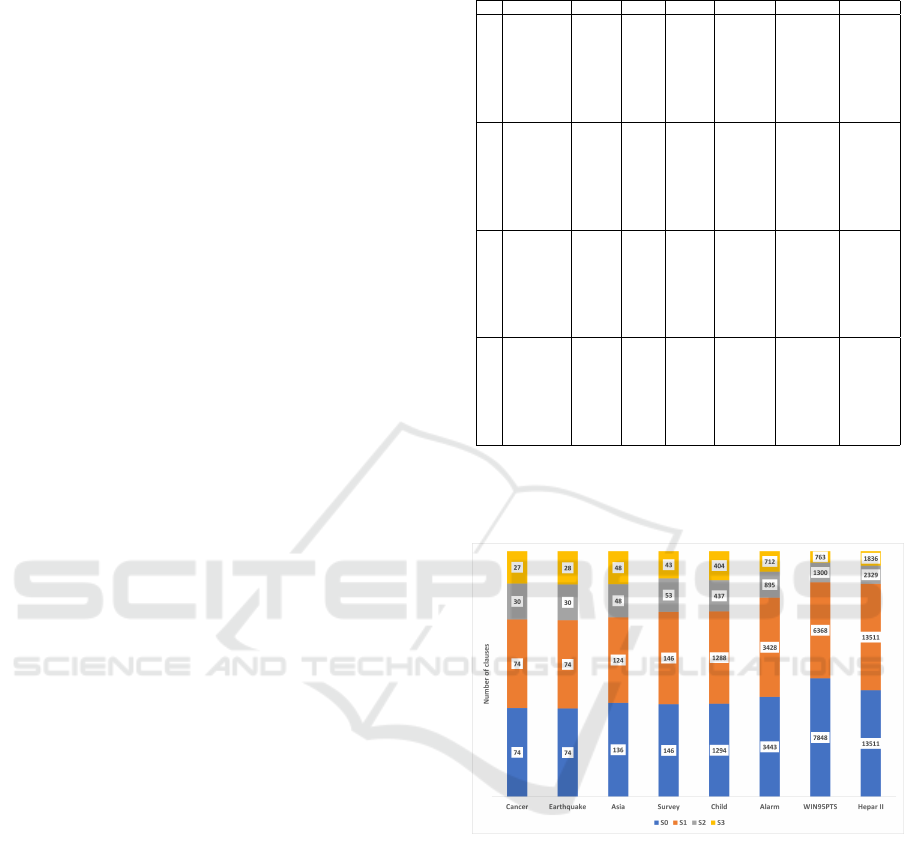
We propose the following graph to compare the

number of clauses for all improvements:

Figure 2: Comparison of the number of clauses.

In this graph, we can see the difference of the

number of clauses between solution S0 and solution

S3. The clauses are drastically reduced. We can see

the improvement of each network in the following

graph:

Improved Encoding of Possibilistic Networks in CNF Using Quine-McCluskey Algorithm

803

Figure 3: Percentage of improvement for the encoding be-

tween solutions S0 and S3.

We can see that the improvement reaches some-

times 90% of deleted clauses with only 10% of re-

maining clauses. We also present the number of nodes

and edges of the d-DNNF graph generated by using

the c2d tool:

(a) Comparison of the number of nodes.

(b) Comparison of the number of edges.

Figure 4: Comparison of the d-DNNF graph.

The results are better with solution S3 (QMC).

The number of clauses is signiﬁcantly reduced. As a

result the graph generated has often fewer nodes and

fewer edges. We compared the c2d computation time

in the global ofﬂine computation time. We obtain the

following graph:

Figure 5: Comparison of c2d computation time and the of-

ﬂine computation time in seconds.

The above ﬁgure shows that the computation time

of c2d is very important compared to the ofﬂine com-

putation time for small and medium networks. That

means that the choice of the compiling tool is very

important for ofﬂine computation.

Then we have compared the computation time for

online inference with two other approaches: the com-

piling of the junction tree of a possibilistic network

(CJT) (Petiot, 2021) and the message-passing (MP)

algorithm adapted to possibilistic networks (Petiot,

2018).

Table 11: Comparison of computation time in seconds.

Networks S3 (s) Cluster Size CJT (s) MP (s)

Asia 0,000124 5 3 0,000186 0,005246

Cancer 0,000087 3 3 0,000092 0,001322

Earthquake 0,000078 3 3 0.000083 0,001463

Survey 0,000192 3 3 0,000212 0,002166

Child 0.007140 16 4 0,014618 0,011534

Alarm 0.116903 26 5 3,293882 0,024094

Win95PTS 0.473409 50 9 4,072174 0,120225

Hepar II 1.102634 57 7 0,293119 0,084800

We present a more synthetic view of the above re-

sults in the following graph. We show for all possi-

bilistic networks the computation time and the num-

ber of parameters.

Figure 6: Comparison of the computation time and network

size.

Our evaluation shows that the solution S3 provides

the best results for small and sometimes medium pos-

sibilistic networks. The best results for large pos-

sibilistic networks are obtained by using message-

passing algorithm. The solution S3 provides globally

better results than the compiling of a junction tree

(CJT). Other improvements are possible. For exam-

ple, A. Darwiche proposes the reduction of the num-

ber of clauses by using eclauses (Chavira and Dar-

wiche, 2005) or the deletion during the encoding of

clauses 2(a) and 2(b) if the variable has no parents.

ICAART 2023 - 15th International Conference on Agents and Artiﬁcial Intelligence

804

6 CONCLUSION

In this research, we have experimented several solu-

tions to reduce the number of clauses during the com-

piling of a possibilistic network. We used the QMC

algorithm to take into account the context-speciﬁc

independence. As a result, we have simpliﬁed the

clauses, even reduced the number of clauses. The use

of c2d tool for the ﬁrst allows us to generate mini-

mized d-DNNF graph. The goal was to obtain the

smallest possible graph to ensure an optimal compu-

tation time.

The proposed approach signiﬁcantly reduces the

number of clauses as well as the computation time

during the encoding of the possibilistic networks. The

online computation time depends on the quality of the

compilation tool used to generate the d-DNNF graph.

Our assessment of inference is satisfactory for small

possibilistic networks. In our future works, we would

like to improve our approach for large networks. We

would like to compare new compiling tools such as

ACE, DSHARP, and D4. We also wish to evaluate at

least two other approaches for compiling possibilistic

networks, the ﬁrst being the logarithmic encoding of

variables and the second the method of factors. Then

we will evaluate quantitative possibilistic networks.

REFERENCES

Beinlich, I. A., Suermondt, H. J., Chavez, R. M., and

Cooper, G. F. (1989). The alarm monitoring system: A

case study with two probabilistic inference techniques

for belief networks. In Hunter, J., Cookson, J., and

Wyatt, J., editors, AIME 89, pages 247–256, Berlin,

Heidelberg. Springer Berlin Heidelberg.

Benferhat, S., Dubois, D., Garcia, L., and Prade, H. (1999).

Possibilistic logic bases and possibilistic graphs. In

Proc. of the Conference on Uncertainty in Artiﬁcial

Intelligence, pages 57–64.

Borgelt, C., Gebhardt, J., and Kruse, R. (2000). Possibilistic

graphical models. Computational Intelligence in Data

Mining, 26:51–68.

Chavira, M. and Darwiche, A. (2005). Compiling bayesian

networks with local structure. IJCAI’05: Proceedings

of the 19th international joint conference on Artiﬁcial

intelligence, pages 1306–1312.

Chavira, M. and Darwiche, A. (2006). Encoding cnfs to em-

power component analysis. Theory and applications

of satisﬁability testing, pages 61–74.

Darwiche, A. (2001). Decomposable negation normal form.

Journal of the Association for Computing Machinery,

(4):608–647.

Darwiche, A. (2002). A logical approach to factoring belief

networks. Proceedings of KR, pages 409–420.

Darwiche, A. (2003). A differential approach to inference

in bayesian networks. J. ACM, 50(3):280–305.

Darwiche, A. (2004). New advances in compiling cnf to

decomposable negation normal form. In ECAI, pages

328–332.

Darwiche, A. and Marquis, P. (2002). A knowledge compi-

lation map. Journal of Artiﬁcial Intelligence Research,

AI Access Foundation, 17:229–264.

Dubois, D., Foulloy, L., Mauris, G., and Prade, H.

(2004). Probability-possibility transformations, trian-

gular fuzzy sets, and probabilistic inequalities. In Re-

liable Computing, pages 273–297.

Dubois, D. and Prade, H. (1988). Possibility theory: An

Approach to Computerized Processing of Uncertainty.

Plenum Press, New York.

Dubois, D., Prade, H., and Sandri, S. A. (1993). On pos-

sibility/probability transformations. R. Lowen and M.

Roubens, Fuzzy Logic: State of the Art, pages 103–

112.

Korb, K. B. and Nicholson, A. E. (2010). Bayesian Artiﬁcial

Intelligence. CRC Press, 2nd edition, Section 2.2.2.

Lauritzen, S. and Spiegelhalter, D. (1988). Local compu-

tation with probabilities on graphical structures and

their application to expert systems. Journal of the

Royal Statistical Society, 50(2):157–224.

McCluskey, E. J. (1956). Minimization of boolean func-

tions. Bell System Technical Journal, 35(6):1417–

1444.

Onisko, A. (2003). Probabilistic Causal Models in

Medicine: Application to Diagnosis of Liver Disor-

ders. Ph.D. Dissertation, Institute of Biocybernetics

and Biomedical Engineering, Polish Academy of Sci-

ence, Warsaw.

Petiot, G. (2018). Merging information using uncertain

gates: An application to educational indicators. Infor-

mation Processing and Management of Uncertainty

in Knowledge-Based Systems. Theory and Founda-

tions - 17th International Conference, IPMU 2018,

adiz, Spain, June 11-15, 2018, Proceedings, Part I,

853:183–194.

Petiot, G. (2021). Compiling possibilistic networks to com-

pute learning indicators. Proceedings of the 13th In-

ternational Conference on Agents and Artiﬁcial Intel-

ligence, 2:169–176.

Raouia, A., Amor, N. B., Benferhat, S., and Rolf, H.

(2010). Compiling possibilistic networks: Alternative

approaches to possibilistic inference. In Proceedings

of the Twenty-Sixth Conference on Uncertainty in Ar-

tiﬁcial Intelligence, UAI’10, pages 40–47, Arlington,

Virginia, United States. AUAI Press.

Scutari, M. and Denis, J.-B. (2014). Bayesian Networks:

with Examples. R. Chapman & Hall.

Spiegelhalter, D. J. and Cowell, R. G. (1992). Learning in

probabilistic expert systems. Proceeding of the 10th

Conference on Uncertainty in Artiﬁcial Intelligence,

pages 447–466.

Zadeh, L. A. (1978). Fuzzy sets as a basis for a theory of

possibility. Fuzzy Sets and Systems, 1:3–28.

Improved Encoding of Possibilistic Networks in CNF Using Quine-McCluskey Algorithm

805