Storage Assignment Using Nested Annealing and Hamming Distances

Johan Oxenstierna

1,4 a

, Louis Janse van Rensburg

, Peter J. Stuckey

2 b

and Volker Krueger

1 c

Dept. of Computer Science, Lund University, Lund, Sweden

Faculty of Information Technology, Monash University, Australia

Optisol, 90 Sippy Downs Dr, QLD, Australia

Kairos Logic AB, Lund, Sweden

Keywords:

Storage Location Assignment Problem, Nested Annealing, Hamming Distances.

Abstract:

The assignment of products to storage locations signiﬁcantly impacts the efﬁciency of warehouse operations.

We propose a multi-phase optimizer for a Storage Location Assignment Problem (SLAP) where solution qual-

ity is based on a distance estimate of future-forecasted order picking. Candidate assignments are ﬁrst sampled

using a Markov Chain accept/reject method. Future-forecasted pick-rounds are then modiﬁed according to the

candidate assignments and solved as Traveling Salesman Problems (TSP). The model is graph-based and gen-

eralizes to any obstacle layout in 2D. Due to the intractability of the SLAP, methods are proposed to speed up

search for strong solution candidates. These include usage of fast function approximation to ﬁnd potentially

strong samples, as well as restarts from local minima. Results show that these methods improve performance

and that total travel distance can be reduced by as much as 30% within 8 hours of CPU-time. We share a public

repository with SLAP instances and corresponding benchmark results on the generalizable TSPLIB format.

1 INTRODUCTION

The Storage Location Assignment Problem (SLAP)

concerns the choice of locations for products in a

warehouse. There are dozens of proposed versions

and optimization methods for the SLAP (Charris

et al., 2018). In this paper we consider SLAP opti-

mization for a standard picker-to-parts scenario where

obstacles can be laid out freely on a 2D plane and

where vehicles (human-controlled or autonomous)

may start and end their paths at any location. A can-

didate solution to the SLAP is an assignment of prod-

ucts to locations. We deﬁne the quality of a candi-

date solution as the aggregate travel distance needed

to complete a given picking-log, i.e., a set of pick-

rounds (sequences of product visits), added to the re-

assignment distance needed to move products to lo-

cations speciﬁed in the candidate solution. A pick-

round is assumed equivalent to a Steiner Traveling

Salesman Problem (TSP) (Valle et al., 2017) where

the origin and destination locations may be different

and where the same location may be revisited by one

or several vehicles. The aggregate TSP distance for

a given assignment is obtained by solving all TSP’s

https://orcid.org/0000-0002-6608-9621

https://orcid.org/0000-0003-2186-0459

https://orcid.org/0000-0002-8836-8816

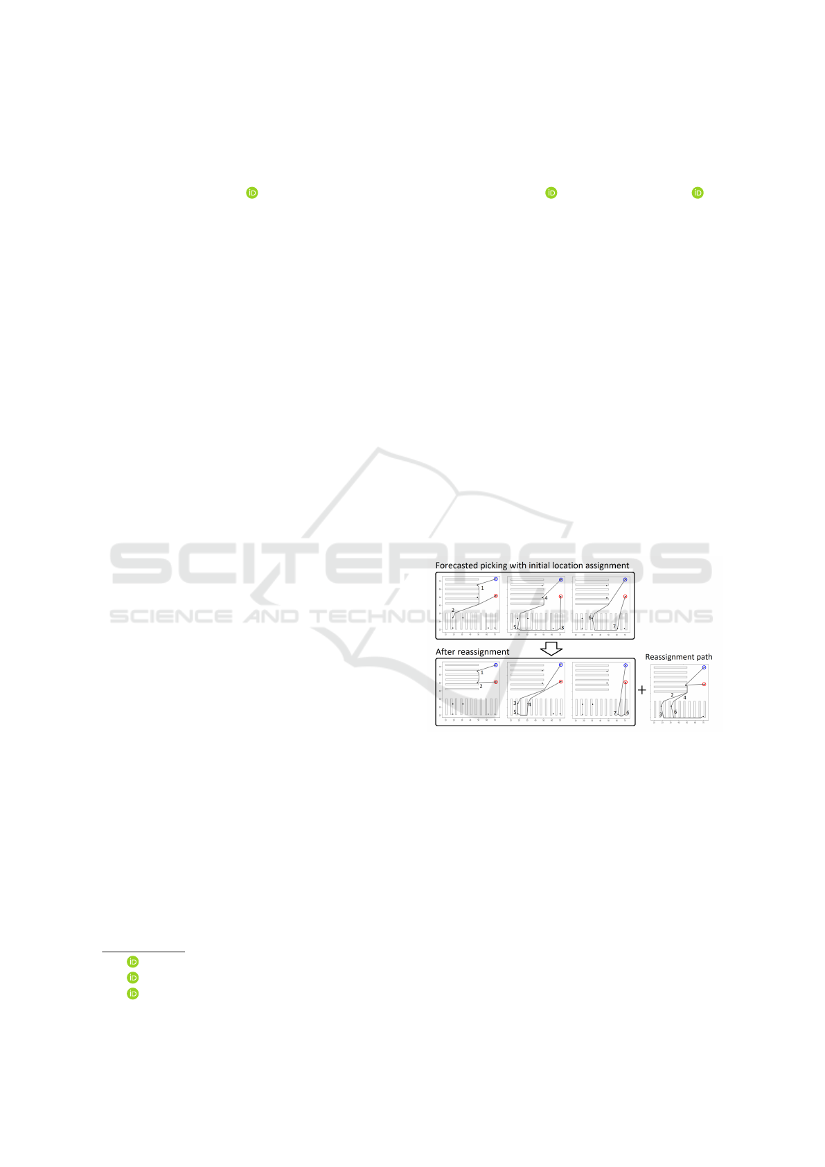
Figure 1: A SLAP example with three pick-rounds (TSP’s)

and an unconventional obstacle-layout. The initial baseline

assignment (top) has a longer picking-log distance com-

pared to a sample/candidate assignment (bottom left). The

reassignment path needed to move the products according

to the sample (bottom right), is longer than any possible

savings concerning the picking-log, however (more pick-

rounds are needed for savings).

in the picking-log according to shortest distance. The

reassignment distance is obtained by optimizing a se-

quence of sub-cycles in a single reassignment path.

We refer to this model as the TSP-based SLAP.

In Section 2 we discuss existing literature on

the SLAP and strengths and weaknesses of various

models, followed by a formulation of the TSP-based

SLAP in Section 4. The proposed model is designed

Oxenstierna, J., van Rensburg, L., Stuckey, P. and Krueger, V.

Storage Assignment Using Nested Annealing and Hamming Distances.

DOI: 10.5220/0011785100003396

In Proceedings of the 12th International Conference on Operations Research and Enterprise Systems (ICORES 2023), pages 94-105

ISBN: 978-989-758-627-9; ISSN: 2184-4372

 2023 by SCITEPRESS – Science and Technology Publications, Lda. Under CC license (CC BY-NC-ND 4.0)

with three main assumptions: 1. The SLAP is static,

meaning that the whole picking-log is given apri-

ori. 2. The picking-log is limited in size, contain-

ing no more than a few hundred products. 3. Prod-

ucts cannot be swapped between pick-rounds. These

assumptions can be criticized for simplifying a re-

alistic SLAP. In a realistic SLAP scenario, strong

location assignments can be assumed to vary dy-

namically based on variable demand. Also, there

may be tens-of-thousands of products within a certain

future-forecasted time-period, instead of a few hun-

dred. Thirdly, the pick-rounds may change their prod-

uct compositions through the future-forecasted time-

period. One argument for the proposed model is that it

is layout-agnostic, meaning that it makes no assump-

tions regarding how racks or other obstacles are laid

out in the warehouse. Another argument for the model

is that it poses a challenging problem even without

the stated simpliﬁcations: The number of possible as-

signments of products to locations is factorial with re-

gard to number of products (assuming a one-to-one

relationship between products and locations). In or-

der to ﬁnd a strong assignment, an equilibrium point

between two adversarial NP-hard problems must be

found: 1. The minimization of TSP’s in the picking-

log, and 2. the minimization of the reassignment cost

needed to move products to their assigned locations.

A ﬁnal argument for the choice of model is the lack

of consensus regarding what should and should not be

included in a basic version of the SLAP, for example

with regard to for benchmark-instances (Charris et al.,

2018). The TSP-based SLAP is our proposal for a

basic version. We offer new public test instances on

the generalizable TSPLIB format (Hahsler and Kurt,

2007) and we invite the community to discuss alter-

native formulations for a basic version of the SLAP.

In Section 5 we introduce our optimization al-

gorithm. It is based on Simulated Annealing and a

Hamming-distance location-swap heuristic. Approx-

imate TSP optimization and restarts from local min-

ima are proposed to improve computational efﬁciency

(cost improvement through CPU-time). In Section 6

we introduce two datasets, including a publicly shared

benchmark instance set, and corresponding compu-

tational results. All used instances are based on a

bi-directional graph, meaning that no uni-directional

travel conventions are assumed. Our contributions are

summarized as follows:

1. A SLAP optimizer using a novel version of the

Simulated Annealing algorithm and experiments

to test its computational efﬁciency.

2. A publicly shared SLAP instance set on

the TSPLIB format and corresponding solu-

tions/results.

2 LITERATURE REVIEW

In this section we discuss how the SLAP has been de-

scribed and optimized in previous work. We particu-

larly refer to the extensive literature review by Charris

et al. (2018). There are several strategies for con-

ducting a storage location assignment. These include

Dedicated, Class-based and Random.

• Dedicated. The locations of products are as-

sumed to never change. This strategy is suitable if

the collection of products does not change much

through time. If human picking is used, this ap-

proach has the advantage that pickers can learn

to associate products with locations, allowing for

speed-ups in picking (Zhang et al., 2019).

• Random. Products can be assigned any location in

the warehouse. This is particularly suitable if the

collection of products changes frequently.

• Class-Based (zoning). Each product is assigned

a class and the warehouse is divided into zones.

Each zone contains one or several classes of prod-

ucts. Class-based storage can incorporate ded-

icated and random strategies for certain zones

and/or classes (Mantel et al., 2007)

The quality of a location assignment can be mod-

eled in several ways. Larco et al. ( 2017), for a human

picking scenario, show that there exists a relationship

between the height which products are placed on and

worker welfare. Worker welfare can be quantiﬁed

by estimating parameters such as “ergonomic load-

ing”, “discomfort” or “expenditure of human energy”

(Charris et al., 2018). For autonomous vehicle or

shuttle based storage and retrieval systems (AVS/R)

there exists a model which has as objective to mini-

mize “energy consumption” (Azadeh et al., 2019).

Another way to judge solution quality is through

datamining, using computations such as support (pick

frequency), conﬁdence (afﬁnity) and lift. These can

also be used to propose SLAP candidate assignments

(Koﬂer et al., 2014; Ming-Huang Chiang et al., 2014;

Zhang et al., 2019). Datamining is primarily focused

on the statistical analysis of products and their rela-

tionships, but it is often combined with order-picking

in a SLAP.

A third proposal studies the effect of trafﬁc con-

gestion. Bottlenecks can be caused if too many

products with high pick-frequency are placed close

to depot, for example. Lee et al. (2020), propose

Correlated and Trafﬁc Balanced Storage Assignment

(C&TBSA), a multi-objective SLAP model which

aims to minimize trafﬁc congestion while also min-

imizing aggregate order -picking cost.

Storage Assignment Using Nested Annealing and Hamming Distances

Order-picking has many variations, depending

on obstacle layout, picking strategy and travel con-

ventions (Charris et al., 2018; Mantel et al., 2007;

Janse van Rensburg, 2019; Yu and Koster, 2009).

Concerning obstacle layout, we distinguish between

two types: Conventional and Unconventional. In the

conventional layout, warehouse racks are assumed to

be organized in Manhattan style blocks with parallel

aisles and cross-aisles. Conventional layouts are used

in the majority of research on both order-picking and

the SLAP (Charris et al., 2018; Koster et al., 2007).

The unconventional layout includes the “ﬁshbone”

and “cascade” layouts (Cardona et al., 2012; Charris

et al., 2018), as well as all other layouts that are not

conventional. Regardless of layout, the picking path

of a vehicle can be formulated as a Traveling Sales-

man Problem (TSP) where paths cannot intersect ob-

stacles (Henn and W

ascher, 2012). For conventional

layouts, the TSP is often optimized using S-shape

or Largest-Gap algorithms (Roodbergen and Koster,

2001). For unconventional layouts, Google OR-tools

or Concorde have been proposed (Oxenstierna et al.,

2022; Janse van Rensburg, 2019).

If a vehicle picks several orders at a time, an Or-

der Batching Problem (OBP) can be formulated. In

the OBP the objective is to assign sets of orders for

the vehicles (an order is a set of products and a batch

is a set of orders). The OBP can be optimized as a

joint problem with the TSP (Gils et al., 2019; Valle

et al., 2017). Proposals to use the OBP to estimate

SLAP solution quality (OBP-based SLAP) include

ubler et al. (2020) and Xiang et al. (2018). The-

oretically, the OBP allows for a strong simulation of

travel in the warehouse, since it includes the search

for product compositions in batch pick-rounds. Using

an OBP within a SLAP also brings noteworthy chal-

lenges, however, since the OBP is highly intractable

(Briant et al., 2020; Oxenstierna et al., 2022).

If batching is not included in the SLAP, heuris-

tics such as Cube per Order Index (COI) (Kal-

lina and Lynn, 1976) and Order Oriented Slotting

(OOS) (Mantel et al., 2007) have been proposed.

COI assumes that products with relatively high pick-

frequency and low volume should be placed close to

depot. COI does not include associations between

products and is therefore mainly suitable for pick-

rounds with few picks, such as pallet-picking or cer-

tain AVS/R systems (Azadeh et al., 2019). OOS, on

the other hand, is speciﬁcally designed for scenar-

ios where orders may contain more than one prod-

uct. Mantel et al. (2007) introduce a Quadratic As-

signment Problem (QAP) heuristic which computes

distances between products and the number of times

products appear in the same order. The quality of a

candidate location assignment can then be estimated

using QAP. Similar methods to OOS are used by

Zulj

et al. (2018), Fontana and Nepomuceno (2017) and

Lee et al. (2020).

The SLAP usecase can be divided into two cate-

gories depending on the number of products that are

to be moved. “Re-warehousing” is the case when

a large proportion of products are moved, whereas

a smaller proportion is moved in “healing” (Koﬂer

et al., 2014). Movements can be conducted in many

ways, each accompanied by a (re)assignment “ef-

fort”. K

ubler et al. (2020) propose the following

(re)assignment effort scenarios:

i Product A is moved to an unoccupied location.

ii Product A swaps location with product B.

iii Product A is moved to a location occupied by

product B. Product B is moved to a new location.

If there is a product C occupying the new loca-

tion the procedure continues until a ﬁnal product

is placed at an empty location.

Scenario (i) comes with the least (re)assignment

effort and the effort grows through scenarios (ii) and

(iii). Apart from travel distance, time used for prod-

uct removal/placement on shelves and administrative

times can be added to the effort computation (K

ubler

et al., 2020).

When it comes to optimization algorithms for the

SLAP, both exact and non-exact methods have been

proposed. The exact algorithms include dynamic pro-

gramming, branch and bound algorithms and Mixed

Integer Linear Programming (MILP) (Charris et al.,

2018). The SLAP search space is often reduced in

scope when exact solutions are sought. These include

restricting the number of locations (Wu et al., 2014),

number of products (Garﬁnkel, 2005; Liu, 1999) or

by only working with conventional warehouse layouts

(Boysen and Stephan, 2013).

More commonly, non-exact heuristic or meta-

heuristic algorithms are used. Proposals include

Particle Swarm Optimization (PSO) (K

ubler et al.,

2020), Genetic and Evolutionary Algorithms (Ene

and

Ozt

urk, 2011; Lee et al., 2020) and Simulated

Annealing (Koﬂer et al., 2014; Zhang et al., 2019).

The SLAP is often optimized in multiple phases using

these methods. One example is to ﬁrst generate candi-

date products for location assignments using datamin-

ing, and then evaluate various candidate assignments

using order-picking optimization (Koﬂer et al., 2014;

Wutthisirisart et al., 2015).

It is challenging to judge optimization results in

previous work due to the multitude of variations in

SLAP models (Charris et al., 2018). For results in-

cluding reassignment costs, conventional warehouse

ICORES 2023 - 12th International Conference on Operations Research and Enterprise Systems

layouts, dynamic picking patterns and meta-heuristic

optimization, Koﬂer et al. (2014) report best sav-

ings around 21%. In a similar scenario, K

ubler et al.

(2020) report best savings around 22%. Excluding re-

assignment costs, Zhang et al. (2019) report best sav-

ings around 18% on simulated data with thousands

of product locations, also using Simulated Annealing.

In a similar setting, for a few hundred products and

using a heuristic two-phase optimizer, Trindade et al.

(2022) report best savings around 33%.

3 SIMULATED ANNEALING AND

MODIFICATIONS

The proposed optimizer (Section 5) is based on Sim-

ulated Annealing (Algorithm 1). A sample function

draws a sample x

i+1

based on a desired distance to a

previous sample x

. The distance is given by some

probability distribution q(x

i+1

), and the distribu-

tion is often chosen to be Normal, so that the dis-

tance between x

i+1

and x

is low with high prob-

ability (Mackay, 1998). The cost

∗

function com-

putes/retrieves the cost ( f

∗

) of the new/previous sam-

ple (the ﬁrst sample is retrieved from memory after

the ﬁrst iteration). The accept probability α

∗

is based

on the solution-space distance function ∆ (which out-

puts a negative value if the new cost is lower than

the previous) and a temperature function T . The tem-

perature enforces high variance at the beginning and

high bias towards the end of optimization (weak new

samples are more often accepted at high temperature)

(Rajasekaran and Reif, 1992). Functions for tempera-

ture T and ∆ are further discussed in Section 5.

The algorithm is a biased random walk and if pro-

portionality between q and f

∗

is large, the random

walk spends more time in regions of local minima.

A known disadvantage of this type of Markov Chain

Monte Carlo (MCMC) method is that each new sam-

ple is correlated to the previous one, risking conver-

gence on weak local minima (Mackay, 1998). Several

methods have been proposed to alleviate this problem,

such as mode-jumping (Tak et al., 2018), Nested An-

nealing (Rajasekaran and Reif, 1992) and Basin Hop-

ping (Wales and Doye, 1997). These methods split the

search space into regions which are then subjected to

local search. Another method is Simulated Annealing

with Restart Strategy (SARS), which restarts the al-

gorithm from a random new sample whenever a “non-

improving” local minimum is found (Yu et al., 2021).

Christen and Fox (2005), propose a method which

can make MCMC algorithms more computationally

efﬁcient, given that there exists a cost function f that

can provide fast and reasonably accurate cost esti-

Algorithm 1: Simulated Annealing.

1: x

: Sample (candidate solution).

2: f

∗

): Ground truth cost of sample x

3: q(x

i+1

): Probability of distance between two

samples.

4: ∆: Cost distance function.

5: N: Number of iterations.

6: T : Temperature function.

7: x

: Initial sample (baseline).

8: for i = 1,...,N do

9: t ← T (i)

10: x

i+1

← sample(q(x

i+1

))

11: f

∗

), f

∗

i+1

) ← cost

∗

i+1

)

12: α

∗

← exp(−c

∆( f

∗

i+1

), f

∗

))/t)

13: u ← U(0,1) // random uniform

14: if u < α

∗

then // sample accepted

15: x

← x

i+1

16: end if

17: end for

mates of f

∗

. They propose to use f to reject new

samples that are unlikely to yield an improvement in

∗

over the previous sample. Using their modiﬁca-

tion, the common MCMC accept method is split into

two parts: Promote ( f

∗

evaluation for a sample with

a strong f ) and accept (update x

for the next itera-

tion to be a sample with a strong f

∗

). In the proposed

algorithm (Section 5), we make use of this concept

and split Simulated Annealing into promotion based

on fast and less accurate TSP optimization in f and

acceptance based on slow and more accurate TSP op-

timization in f

∗

4 PROBLEM FORMULATION

4.1 Objective Function

The objective in the TSP-based SLAP is to minimize

the aggregate travel distance to:

1. Complete a given set of pick-rounds B.

2. Carry out any proposed locations reassignments

in a single reassignment path R .

Each pick-round b ∈ B is a list of products. The set of

all locations (including pick-locations, origin and des-

tinations and obstacle corners in 2D Cartesian space)

is denoted L and the set of all pick-locations is de-

noted L(P ). The set of all products found in B is

denoted P . Each product p ∈ P is a tuple consist-

ing of a unique key (Stock Keeping Unit), a location

l(p) ∈ L(P ) and a positive quantity. Each pick loca-

tion is a tuple consisting of a unique key, a capacity

Storage Assignment Using Nested Annealing and Hamming Distances

and a location (represented as a node key in a graph).

A product is located at strictly one location and a loca-

tion stores strictly one product. A product is allowed

to move from its initial location to a new one as long

as the new location’s capacity is not exceeded.

A SLAP solution candidate (also referred to as

sample or assignment) is represented as permutation

vector x ∈ X, where the elements are enumerated

product keys and the indices are enumerated loca-

tion keys. For an example warehouse with 3 loca-

tions, sample x = [2, 1,3] means that product 2 is as-

signed location 1, 1 assigned 2 and 3 assigned 3. Each

x contains permutation integers in the range [1,m],

2 ≤ m ≤ |P | and each permutation has ground truth

cost f

∗

(solution value) (see Equation 1). m denotes

the number of products that are subject to location

change, and it can be set manually to limit the search

space (Section 5). Sample x

represents the base-

line product location assignment (the inital locations

of the products). The cost of all subsequent samples

will be compared against the initial baseline cost of

. The minimization of the picking-log and reassign-

ment distance is as follows,

argmin

((

∑

b∈B

D(b)) + λD(R )) (1)

The objective is to ﬁnd a sample x such that picking-

log distance

∑

b∈B

D(b) and reassignment distance

D(R ) are minimized. The factor λ allows us to weigh

the two costs. Below we show how each of them is

computed.

4.2 Picking-Log Distance

The distance of all pick-rounds in picking-log B

is computed as

∑

b∈B

D(b). D(b) is the distance

of the solution to the Traveling Salesman Problem

(TSP) represented by product locations in b: D(b) =

l(origin),l(p

)

+ d

l(p

|b|

),l(destination)

∑

l(p

),l(p

)

, j =

i + 1,0 < i < |b|, where d

l(p

),l(p

)

denotes the

distance between the locations of p

, p

∈ b, and

where d

l(origin),l(p

)

connects an origin location and

l(p

|b|

),l(destination)

a destination location to the path.

The location of a product l(p

) is obtained from an in-

dex in the location assignment sample x. We assume

shortest distances and corresponding shortest paths

(needed if visualization is sought) between pairs of lo-

cations are queryable from Random Access Memory

(RAM). All these shortest distances and paths are pre-

computed using the Floyd-Warshall algorithm on a bi-

directed graph, using a warehouse digitization process

beyond the scope of this paper (Janse van Rensburg,

2019). We allow the origin and destination locations

in the pick-rounds to be any locations in L (this is

sometimes referred to as Multi-Depot TSP or Dial-

a-ride Problem). In Section 5 we describe how TSP

optimization works for the multi-depot requirement.

4.3 Reassignment Distance

Reassignment path R and its distance D(R ) is based

on direct and indirect exchange scenarios (scenarios

(ii) and (iii) (Section 2) with the following assump-

tions: Since there are an equal amount of products

and locations in the formulated SLAP, scenarios (ii)

and (iii) are a bijection of products and locations. We

also assume three enumeration types for the bijection:

Direct exchange, e.g. x

= [1, 2] to x

= [2, 1] (prod-

uct 2 goes to location 1 and 1 goes to 2), indirect ex-

change, e.g. x

= [1, 2,3] to x

= [3, 1,2] (1 goes to 2,

2 goes to 3 and 3 goes to 1), or a combination of both.

We also assume direct and indirect exchanges can be

carried out in a single path without intermediate stops

at the depot. Algorithm 2 shows how a single reas-

signment path can be built and optimized just from

information in initial assignment x

and subsequent

sample x

i+1

(generated during optimization).

Algorithm 2: Reassignment Path Optimization.

1: x

: Initial assignment (baseline solution)

2: x: Sample obtained during optimization

3: x

← copy(x)

4: D(R

best

) ← ∞

5: for i = 1,...,K do // optimization iterations.

6: R ← list()

7: while x

not empty do

8: r ← list()

9: while not completed(r) do

10: r.add(x,x

) // add to sub-cycle

11: end while

12: R + = r

13: end while

14: shufﬂe and ﬂatten(R )

15: D(R

best

) ← update best(R , R

best

)

16: end for

r denotes a sub-cycle of locations (sequence that

starts and ends at the same location). r.add(x,x

)

has two cases: 1. If r is empty, a random new element

is removed from x

and its initial location (the index

for that product in x

) is added to r. 2. If r is not

empty, the new location of the last added product in r

is ﬁrst found in x and added to r. The product which

sits at that “next” location is found in x

, matched in

and then removed from x

. If the added location to r

is equivalent to the ﬁrst one in r, the sub-cycle is com-

pleted and r is added to R . After x

is emptied, R is

ﬁrst randomly shufﬂed and then ﬂattened (the inner

ICORES 2023 - 12th International Conference on Operations Research and Enterprise Systems

lists of subcycles are converted into a single list). The

distance D(R ) is then computed as the sum of all lo-

cation to location distances in R , added with the dis-

tance from an origin depot location to the ﬁrst location

in R and the last location in R to a destination depot

location. At each iteration, the update best(R ,R

best

)

function updates the lowest minimum found by com-

paring distance D(R ) and distance D(R

best

). For Al-

gorithm 1 and Algorithm 3 (below), D(R ) is included

in the cost

∗

and cost functions.

R is a solution to a constrained, linked-list TSP

where a product is dropped off and another product

picked up at each location. The vehicle conducting

the reassignment path is assumed to be able to carry

the whole quantity of one product. A model of the re-

assignment path involving vehicle-capacities, enforc-

ing return trips to depot when a product quantity ex-

ceeds capacity, is left for future work.

5 OPTIMIZATION ALGORITHM

5.1 SLAP Markov Chain Monte Carlo

(MCMC)

We formulate Markovian sampling distribution q

which is capable of proposing a distance from a sam-

ple x

to a next sample x

i+1

such that Equation 1 is

minimized. For this to be possible, there must ex-

ist a proportionality between the cost expressed in

Equation 1 and q. We hypothesize that such pro-

portionality exists between the cost and a q involv-

ing a Hamming distance heuristic. Hamming distance

measures the distance between permutations and it

involves counting of non-identical elements between

the permutations (Rathod et al., 2016). The following

sampling distribution is then proposed (loosely based

on bounds proposed by Christen and Fox (2005)):

q(x

i+1

) = e

−CH

i+1

)

(2)

where C and P are hyperparameters in R

, and H

denotes Hamming distance between two samples.

The Hamming distance gives the number of loca-

tion changes compared to the previous sample, and

the number is determined by the q probability. In

the remainder of this section, we propose to use this

sampling function within Algorithm 1. We also pro-

pose methods which may improve computational ef-

ﬁciency (cost reduction through CPU-time) of Algo-

rithm 1.

5.2 TSP Optimization and Caching

In order to compute the quality of a SLAP solution

candidate, TSP optimization is required. For optimal

TSP solutions we use Concorde

(Applegate et al.,

2002). For approximate TSP solutions we use OR-

tools

(Kruk, 2018). In order to limit the CPU-time

of OR-tools, its solution limit parameter is set to 500,

which is the maximum number of candidate TSP so-

lutions that it is allowed to evaluate before termi-

nating. Capability to handle multi-depot scenarios

is added by modifying the input distance matrix by

adding a dummy location whose distance is zero to

the origin and destination, and whose other distances

are set to inﬁnite.

Given sampling function q, it is evident that only a

subset of the pick-rounds in the picking-log are going

to be affected by any given product to location assign-

ment (pick-rounds will often not contain reassigned

products). Instead of re-optimizing the same pick-

rounds where no products have changed location, we

instead cache optimal and approximate cost for each

pick-round once computed. For any pick-round, the

saved costs are then queried until one or several prod-

uct locations are changed.

5.3 Nested Annealing

Algorithm 1 can potentially be made more computa-

tionally efﬁcient if there exists a function f which can

quickly estimate f

∗

(Section 3). The modiﬁcation is

shown in Algorithm 3.

After a sample x

i+1

is generated, its cost is esti-

mated using OR-tools. If the sample passes the pro-

mote ﬁlter, cost

∗

is computed using Concorde. The

cost and cost

∗

functions include reassignment dis-

tance D(R ) (Algorithm 2). Since Algorithm 2 does

not guarantee optimality for D(R ), cost

∗

does not

guarantee optimality either, and hence we refer to f

∗

as “more accurate” rather than optimal. Note that

hyperparameters c

∈ R

may be set differently.

Christen and Fox (2005) suggest setting c

> c

that the promotion of a sample is less likely than

the acceptance of a promoted sample. The temper-

ature function T is assumed to be a shifted and scaled

reverse sigmoid (decreasing) that gives temperatures

in range [1,0]. The pairwise solution-space distance

function ∆ is assumed to be a shifted and scaled sig-

moid that gives values in range [0,1]. Nested An-

nealing was ﬁrst introduced by Rajasekaran and Reif

https://math.uwaterloo.ca/tsp/concorde/downloads/d

ownloads.htm, collected 27-05-2022.

https://developers.google.com/optimization/routing/t

sp, collected 12-06-2022.

Storage Assignment Using Nested Annealing and Hamming Distances

Algorithm 3: Nested Annealing (based on computational

efﬁciency in cost estimation).

1: x

: Sample (candidate solution)

2: f (x

): Less accurate fast cost estimate

3: f

∗

): More accurate slow cost estimate

4: q(x

i+1

): Probability of distance between two

samples

5: α: Probability that sample x

i+1

is promoted

6: α

∗

: Probability that sample x

i+1

is accepted

7: ∆: Cost distance function

8: N: Number of iterations

9: T : Temperature function

10: x

: Initial assignment sample (baseline)

11: for i = 1,...,N do

12: t ← T (i)

13: x

i+1

← sample(q(x

i+1

))

14: f (x

), f (x

i+1

) ← cost(x

i+1

)

15: α ← exp(−c

∆( f (x

i+1

), f (x

))/t)

16: u ← U(0, 1) // random uniform

17: if u < α then // sample promoted

18: f

∗

), f

∗

i+1

) ← cost

∗

i+1

)

19: α

∗

← exp(−c

∆( f

∗

i+1

), f

∗

))/t)

20: u ← U(0, 1)

21: if u < α

∗

then // sample accepted

22: x

← x

i+1

23: end if

24: end if

25: end for

(1992), but they do not use function approximation

and base the nesting on variable set temperatures in

local search regions. Algorithm 3 provides an alter-

native nesting strategy, based on a tradeoff between

predictive speed and accuracy.

5.4 Restarts

Due to the large search space of the SLAP, the MCMC

sampling function x

i+1

← sample(q(x

i+1

)), may

beneﬁt from occasional restarts (Section 2). Yu et

al. (2021), propose restarts from randomly generated

samples. Their test-problems do not include reassign-

ment distances, however, and in the SLAP, randomly

generated samples can be expected to have a signif-

icantly higher cost than x

, due to reassignment dis-

tance D(R ). We thus propose restarts from local min-

ima. The best minimum found through optimization

is denoted x

best

and it is used as restart sample with an

increasing probability. Forcing restarts from x

best

motivated because its local neighbourhood cannot be

extensively searched for in any but the smallest SLAP

test-instances. Another minimum is denoted x

lowR

and it is used as restart sample with a decreasing prob-

ability (distributions proposed in Section 6). Forcing

restarts from x

lowR

is designed to target a low reas-

signment distance D(R ). The ﬁrst such local min-

imum is x

lowR

= x

, whose D(R ) = 0. x

lowR

= x

can be assumed to be a strong local minimum, due to

its lack of reassignment distance, but after f

∗

) has

been conclusively beaten, x

lowR

is updated at regular

intervals to a previously generated sample which has

a relatively low f

∗

cost and D(R ). In Section 6 we

present optimization results with and without restarts

from x

best

and x

lowR

6 EXPERIMENTS

6.1 Overview

We carry out experiments to investigate the following

topics with regard to computational efﬁciency (cost

improvement through CPU-time):

1. Utility of Hamming-distance based sampling (q).

2. Utility of restarts.

3. Algorithm 1 compared to Algorithm 3.

4. Other features (such as layout and number of

products and pick-rounds).

All experiments are carried out using Intel Core

i7-4700MQ, 2.40GHz, 4 cores and Python3 (with

heavy use of Cython) and C.

6.2 Parameters

For all experiments, the number of products open for

location reassignment (m) is set to be equivalent to

the number of products in the test-instance. The num-

ber of reassignment path optimization iterations (K

in Algorithm 2) is set to 300. After optimization

has completed, the reassignment path is re-optimized

with K set to 10000. The accept probability computa-

tion is set to be equivalent between Algorithm 1 and 3

= 1 and equivalent ∆ and T functions). The ∆

function is set to approach 1 when the ratio of the

distance between a new sample and a previous sam-

ple exceeds 1.05: If a new sample has a distance 5%

higher than the previous sample, it is unlikely to be

promoted and/or accepted. c

in Algorithm 3 is set

to 2, which makes it more difﬁcult for a sample to

be promoted than accepted once promoted. The re-

verse sigmoid probability distribution q, which gives

the number of location changes between a new and a

previous sample, is set to approach zero when number

of location changes exceeds 20. For all experiments

where a restart strategy is used, sample x

i+1

can be

built from either x

, x

best

or x

lowR

(Section 5). The

ICORES 2023 - 12th International Conference on Operations Research and Enterprise Systems

100

probability to pick one of the latter two is governed

by a sigmoid and reverse sigmoid, respectively, with

probabilities in range [0,0.2] and [0.2, 0], stretched

over N iterations. In all iterations where neither of

the latter two is picked, x

is used (no restarts). The

total number of iterations and/or CPU-time is set de-

pending on dataset (see below). λ is set to 1 in all

experiments.

6.3 Datasets

The following two datasets are used:

• 266 TSPLIB instances

modiﬁed for the SLAP

and shared in a public repository

. These in-

stances include 6 different types of warehouse

layouts (including one with no obstacles), all

modeled as bi-directional graphs (without uni-

directional travel-conventions). The number of

products open for location reassignment vary be-

tween 5-427 in these instances. The initial loca-

tions for all products (baseline assignment x

) in

these instances is selected using a random uniform

distribution. Solution proposals are uploaded for

each of these instances using Algorithm 3 after a

maximum of 20000 iterations (N). Experiments

to test utility of Hamming distances and restarts

are conducted on this dataset.

• A real warehouse with a conventional layout and

without any uni-directional travel conventions.

The provided picking log for this warehouse in-

cludes 260 unique products and 260 product loca-

tions. There are 200 pick-rounds and most prod-

ucts are picked in several pick-rounds. The ex-

periments where Algorithm 1 and 3 are compared

are run on this dataset. Algorithm 1 and 3 are

run 10 times each on this dataset, with varying

random seeds and a maximum CPU-time set to 8

hours. For a discussion regarding how often stor-

age (re)assignments can be expected to be con-

ducted (which may guide the choice of optimiza-

tion time), see Section 2.

In both datasets, the capacity of all locations is as-

sumed to be identical, meaning that any product can

be placed at any location. We compare costs of sam-

ples against the baseline x

, where each product is

ﬁxed to its initial location, where optimal picking

costs are computed in D(B) and where D(R ) = 0.

https://github.com/johanoxenstierna/OBP/instances,

collected 19-10-2022.

https://github.com/johanoxenstierna/L40 266, col-

lected 14-11-2022

Figure 2: The total number of product location reassign-

ments needs to be large to achieve the best total travel costs

in f

∗

best

6.4 Experimental Results

6.4.1 Utility of Hamming-Distance Based

Sampling

Results show that many location reassignments are

needed to reach the best reductions in travel cost (Fig-

ure 2). Also, more reduction in cost is achieved when

the Hamming distance (number of location changes)

between a previous sample and a new one is rela-

tively low (Figure 3). On average, the cost of sam-

ple f

∗

i+1

) is more reduced compared to a previ-

ous sample f

∗

) if fewer location changes are at-

tempted. This result empirically validates the Ham-

ming distance distribution q(x

i+1

) and its bias to-

ward fewer location changes (Equation 2).

6.4.2 Utility of Restarts

Aggregated results with and without restarts (Section

5) are shown in Figure 4. Given the same amount of

optimization iterations (N = 30000) on the real ware-

house dataset, the best results for both Algorithm 1

and 3 are obtained using restarts. Restarts enforce

revisits to local minima with relatively short total

travel costs f

∗

or reassignment paths D(R ) (Section

5). Since fewer reassignments mean that fewer pick-

rounds contain products whose locations change, TSP

optimization CPU-time is signiﬁcantly lower when

restarts are used. This is achieved by the caching

of TSP costs (Section 5). Furthermore, few reassign-

ments mean that the optimization of the reassignment

path requires less CPU-time to reach a strong solu-

tion. As can be observed, Algorithm 1 and 3 without

restarts (lighter blue and green) quickly jump up in

cost. This is mainly attributed to the relatively low

cost in initial assignment x

, where D(R ) = 0, which

Storage Assignment Using Nested Annealing and Hamming Distances

101

Figure 3: Distribution (violin) plot showing number of loca-

tion changes against picking-log distance D(B) (blue) and

reassignment distance D(R ) (orange) when moving from a

previous sample to a new sample. The mean cost of both

D(B) and D(R ) increase when more location changes are

attempted in new samples. This plot excludes any x

and

i+1

pairs where either were restarts back to a local mini-

mum.

Figure 4: Algorithm 1 and Algorithm 3 with and without

restarts for 30000 iterations on the real warehouse dataset.

The costs shown are for f

∗

i+1

is never revisited once stepped away from and never

improved on (without restarts).

6.4.3 Algorithm 1 Compared to Algorithm 3

Algorithm 3 (Nested Annealing with restarts) out-

performs Algorithm 1 (Simulated Annealing with

restarts) within the given CPU-time (Figure 5). The

Markov chain in Algorithm 3 is more biased com-

pared to the one in Algorithm 1, due to more sam-

ples being rejected. Algorithm 1 accepts more sam-

ples with high cost, which may lead to the discovery

of more attractive search regions, if given more CPU-

time than 8 hours.

Figure 5: Aggregate CPU-time against shortest total travel

cost ( f

∗

best

)) on the real warehouse dataset (20 optimiza-

tion runs): Blue is Algorithm 1, green is Algorithm 3 and

red is the cost of baseline assignment x

(100%). The shad-

owed areas represent 95% conﬁdence intervals.

6.4.4 Other Features

Aggregate averages of results on the generated in-

stances and Algorithm 3 are shown in Table 1 (Ap-

pendix). The elements for columns f (x

), f

∗

f (x

i+1

), f

∗

i+1

), f

∗

best

), D(R)

D(R)

300

are all

shown as percentages against the distance of the base-

line cost f

∗

) (100%). D(R)

and D(R)

300

denote

the distance of the reassignment path after Algorithm

2 has been run for 1 and 300 iterations, respectively.

The rows are aggregated averages based on number of

products shown in column 1, from a total of 5279885

samples on the generated instance dataset (with 3-12

minutes CPU-time on each instance). One interesting

result in Table 1 is that the predictive quality of f (x

)

is almost identical to f

∗

). OR-tools delivers very

strong solutions to the given picking-log B, which is

explainable since pick-rounds b ∈ B rarely exceed 15

locations in length. This means that the strong perfor-

mance of Algorithm 3 with restarts (Figure 4), may

be achievable by Algorithm 1 set up with restarts and

with a higher accept threshold c

(instead of using the

promote ﬁlter), at least for the used datasets.

No correlation was found between the warehouse

layout (the six ones in the generated instance set)

and features such as total cost improvement, reassign-

ment distance and/or number of ﬁnal proposed loca-

tion reassignments. This is explainable since both

TSP-optimizers (OR-tools and Concorde) and the re-

assignment path optimizer (Algorithm 2) are layout-

agnostic (Section 1).

7 CONCLUSION

An optimization model for the Storage Assignment

Location Problem (SLAP) was proposed. In the TSP-

ICORES 2023 - 12th International Conference on Operations Research and Enterprise Systems

102

based SLAP, products cannot be swapped between

pick-rounds and future-forecasted picking is assumed

to be static. Furthermore, the warehouse rack layout

is assumed to have any conﬁguration in 2D. An opti-

mizer based on Simulated Annealing, to provide solu-

tions to the TSP-based SLAP, was proposed. The op-

timizer generates assignment samples using a Ham-

ming distance function and two accept ﬁlters. A

restart heuristic, which forces occasional revisits to

local minima, is also used. Since products cannot be

reassigned to new locations for free, the distance of a

reassignment path is added to the cost of any gener-

ated sample.

Two datasets were used to evaluate the proposed

optimizer: A real warehouse dataset and a set of pub-

licly shared test-instances on a generalizable format.

The modiﬁcations to standard Simulated Annealing

were found to be motivated and the best cost savings,

of around 30%, were achieved after 8 hours of CPU-

time. Overall this result is in line with results in prior

work where strong assumptions are made with re-

gard to warehouse layout (but where dynamicity may

be assumed or where number of products is larger)

(Koﬂer et al., 2014; K

ubler et al., 2020; Trindade

et al., 2022).

For future work, heuristics to increase bias in the

proposed algorithm could be investigated. These in-

clude zoning, where products are set up to be drawn

to certain areas in the warehouse. Another heuris-

tic is λ (Section 4), and it can be deﬁned to be ad-

justed dynamically (instead of being a constant), to

potentially improve optimization performance and/or

to reﬂect a more realistic division between the cost

of picking and reassignment of products. For exam-

ple, λ could be set to start at a low value and then

to grow linearly. Setting it to a low value initially

would prevent many samples from being rejected due

to the clear relationship between few number of reas-

signments and low cost reduction (Figure 2). Another

proposal involves analysis of the future-forecast pick-

ing log and how it relates to potential savings. Zhang

et al. (2019) and Koﬂer et al. (2014) use datamin-

ing heuristics to show that reassignment ”potential”

is correlated to the way in which products in pick-

rounds are distributed. It is challenging to make use

of such heuristics to make concrete proposals for re-

assignments in a Markov chain, however. The TSP-

based SLAP is highly intractable, even though it is a

simpliﬁcation of storage assignment in realistic use-

cases.

ACKNOWLEDGEMENTS

This work was partially supported by the Wallen-

berg AI, Autonomous Systems and Software Program

(WASP) funded by the Knut and Alice Wallenberg

Foundation. We also convey thanks to Kairos Logic

AB for software.

REFERENCES

Applegate, D., Cook, W., Dash, S., and Rohe, A. (2002).

Solution of a Min-Max Vehicle Routing Problem. IN-

FORMS Journal on Computing, 14:132–143.

Azadeh, K., De Koster, R., and Roy, D. (2019). Robotized

and Automated Warehouse Systems: Review and Re-

cent Developments. Transportation Science, 53.

Boysen, N. and Stephan, K. (2013). The deterministic

product location problem under a pick-by-order pol-

icy. Discrete Applied Mathematics, 161(18):2862 –

2875.

Briant, O., Cambazard, H., Cattaruzza, D., Catusse, N.,

Ladier, A.-L., and Ogier, M. (2020). An efﬁcient

and general approach for the joint order batching and

picker routing problem. European Journal of Opera-

tional Research, 285(2):497 – 512.

Cardona, L. F., Rivera, L., and Mart

ınez, H. J. (2012). An-

alytical study of the Fishbone Warehouse layout. In-

ternational Journal of Logistics Research and Appli-

cations, 15(6):365–388.

Charris, E. et al. (2018). The storage location assignment

problem: A literature review. International Journal of

Industrial Engineering Computations, 10.

Christen, J. A. and Fox, C. (2005). Markov Chain Monte

Carlo Using an Approximation. Journal of Computa-

tional and Graphical Statistics, 14(4):795–810.

Ene, S. and

Ozt

urk, N. (2011). Storage location assignment

and order picking optimization in the automotive in-

dustry. The International Journal of Advanced Manu-

facturing Technology, 60:1–11.

Fontana, M. E. and Nepomuceno, V. S. (2017). Multi-

criteria approach for products classiﬁcation and

their storage location assignment. The Interna-

tional Journal of Advanced Manufacturing Technol-

ogy, 88(9):3205–3216.

Garﬁnkel, M. (2005). Minimizing multi-zone orders in the

correlated storage assingment problem. PhD Thesis,

School of Industrial and Systems Engineering, Geor-

gia Institute of Technology.

Gils, T. v., Caris, A., Ramaekers, K., and Braekers, K.

(2019). Formulating and solving the integrated batch-

ing, routing, and picker scheduling problem in a real-

life spare parts warehouse. European Journal of Op-

erational Research, 277(3):814–830.

Hahsler, M. and Kurt, H. (2007). TSP – Infrastructure for

the Traveling Salesperson Problem. Journal of Statis-

tical Software, 2:1–21.

Henn, S. and W

ascher, G. (2012). Tabu search heuristics for

the order batching problem in manual order picking

Storage Assignment Using Nested Annealing and Hamming Distances

103

systems. European Journal of Operational Research,

222(3):484–494. Publisher: Elsevier.

Janse van Rensburg, L. J. v. (2019). Artiﬁcial intelli-

gence for warehouse picking optimization - an NP-

hard problem. Master’s thesis, Uppsala University.

Kallina, C. and Lynn, J. (1976). Application of the Cube-

per-Order Index Rule for Stock Location in a Distri-

bution Warehouse. Interfaces, 7(1):37–46.

Koﬂer, M., Beham, A., Wagner, S., and Affenzeller, M.

(2014). Afﬁnity Based Slotting in Warehouses with

Dynamic Order Patterns. (Advanced Methods and

Applications in Computational Intelligence):123–143.

Koster, R. d., Le-Duc, T., and Roodbergen, K. J. (2007).

Design and control of warehouse order picking: A lit-

erature review. European Journal of Operational Re-

search, 182(2):481 – 501.

Kruk, S. (2018). Practical Python AI Projects: Mathemat-

ical Models of Optimization Problems with Google

OR-Tools. Apress.

ubler, P., Glock, C., and Bauernhansl, T. (2020). A new

iterative method for solving the joint dynamic storage

location assignment, order batching and picker rout-

ing problem in manual picker-to-parts warehouses.

147:106645.

Larco, J. A., Koster, R. d., Roodbergen, K. J., and Dul, J.

(2017). Managing warehouse efﬁciency and worker

discomfort through enhanced storage assignment de-

cisions. International Journal of Production Re-

search, 55(21):6407–6422.

Lee, I. G., Chung, S. H., and Yoon, S. W. (2020). Two-stage

storage assignment to minimize travel time and con-

gestion for warehouse order picking operations. Com-

puters & Industrial Engineering, 139:106129.

Liu, C.-M. (1999). Clustering techniques for stock location

and order-picking in a distribution center. Computers

& Operations Research, 26(10):989–1002.

Mackay, D. J. C. (1998). Introduction to Monte Carlo Meth-

ods. In Learning in Graphical Models.

Mantel, R. et al. (2007). Order oriented slotting: A new as-

signment strategy for warehouses. European Journal

of Industrial Engineering, 1:301–316.

Ming-Huang Chiang, D., Lin, C.-P., and Chen, M.-C.

(2014). Data mining based storage assignment heuris-

tics for travel distance reduction. Expert Systems,

31(1):81–90. Publisher: Wiley Online Library.

Oxenstierna, J., Malec, J., and Krueger, V. (2022). Analysis

of Computational Efﬁciency in Iterative Order Batch-

ing Optimization. In Proceedings of the 11th Interna-

tional Conference on Operations Research and Enter-

prise Systems - ICORES,, pages 345–353. SciTePress.

Rajasekaran, S. and Reif, J. H. (1992). Nested annealing: a

provable improvement to simulated annealing. Theo-

retical Computer Science, 99(1):157–176.

Rathod, A. B., Gulhane, S. M., and Padalwar, S. R. (2016).

A comparative study on distance measuring approches

for permutation representations. In 2016 IEEE inter-

national conference on advances in electronics, com-

munication and computer technology (ICAECCT),

pages 251–255. IEEE.

Roodbergen, K. J. and Koster, R. (2001). Routing methods

for warehouses with multiple cross aisles. Interna-

tional Journal of Production Research, 39(9):1865–

1883.

Tak, H., Meng, X.-L., and Dyk, D. A. v. (2018). A Re-

pelling–Attracting Metropolis Algorithm for Multi-

modality. Journal of Computational and Graphical

Statistics, 27(3):479–490.

Trindade, M. A. M., Sousa, P., and Moreira, M. (2022).

Ramping up a heuristic procedure for storage loca-

tion assignment problem with precedence constraints.

Flexible Services and Manufacturing Journal, 34.

Valle, C., Beasley, J. E., and da Cunha, A. S. (2017). Opti-

mally solving the joint order batching and picker rout-

ing problem. European Journal of Operational Re-

search, 262(3):817–834.

Wales, D. J. and Doye, J. P. K. (1997). Global Optimiza-

tion by Basin-Hopping and the Lowest Energy Struc-

tures of Lennard-Jones Clusters Containing up to 110

Atoms. Journal of Physical Chemistry A, 101:5111–

5116.

Wu, J., Qin, T., Chen, J., Si, H., and Lin, K. (2014). Slot-

ting Optimization Algorithm of the Stereo Warehouse.

In Proceedings of the 2012 2nd International Confer-

ence on Computer and Information Application (IC-

CIA 2012), pages 128–132. Atlantis Press.

Wutthisirisart, P., Noble, J. S., and Chang, C. A. (2015). A

two-phased heuristic for relation-based item location.

Computers & Industrial Engineering, 82:94–102.

Xiang, X., Liu, C., and Miao, L. (2018). Storage as-

signment and order batching problem in Kiva mo-

bile fulﬁlment system. Engineering Optimization,

50(11):1941–1962.

Yu, M. and Koster, R. B. M. d. (2009). The impact of or-

der batching and picking area zoning on order pick-

ing system performance. European Journal of Opera-

tional Research, 198(2):480 – 490.

Yu, V. F., Winarno, Maulidin, A., Redi, A. A. N. P., Lin,

S.-W., and Yang, C.-L. (2021). Simulated Annealing

with Restart Strategy for the Path Cover Problem with

Time Windows. Mathematics, 9(14).

Zhang, R.-Q. et al. (2019). New model of the storage loca-

tion assignment problem considering demand corre-

lation pattern. Computers & Industrial Engineering,

129:210–219.

Zulj, I., Glock, C. H., Grosse, E. H., and Schneider, M.

(2018). Picker routing and storage-assignment strate-

gies for precedence-constrained order picking. Com-

puters & Industrial Engineering, 123:338–347.

ICORES 2023 - 12th International Conference on Operations Research and Enterprise Systems

104

APPENDIX

Table 1: Aggregate averages of results from 5279885 generated samples for optimization runs on the 266 publicly

shared instances. The results are aggregated based on ranges of number of products (the ﬁrst column).

Storage Assignment Using Nested Annealing and Hamming Distances

105