Interpretable Machine Learning for Modelling and Explaining Car

Drivers’ Behaviour: An Exploratory Analysis on Heterogeneous Data

Mir Riyanul Islam

∗ a

, Mobyen Uddin Ahmed

and Shahina Begum

Artiﬁcial Intelligence and Intelligent Systems Research Group, School of Innovation Design and Engineering,

alardalen University, Universitetsplan 1, 722 20 V

aster

as, Sweden

∗

Corresponding Author

Keywords:

Artiﬁcial Intelligence, Driving Behaviour, Feature Attribution, Evaluation, Explainable Artiﬁcial Intelligence,

Interpretability, Road Safety.

Abstract:

Understanding individual car drivers’ behavioural variations and heterogeneity is a signiﬁcant aspect of devel-

oping car simulator technologies, which are widely used in transport safety. This also characterizes the hetero-

geneity in drivers’ behaviour in terms of risk and hurry, using both real-time on-track and in-simulator driving

performance features. Machine learning (ML) interpretability has become increasingly crucial for identifying

accurate and relevant structural relationships between spatial events and factors that explain drivers’ behaviour

while being classiﬁed and the explanations for them are evaluated. However, the high predictive power of ML

algorithms ignore the characteristics of non-stationary domain relationships in spatiotemporal data (e.g., de-

pendence, heterogeneity), which can lead to incorrect interpretations and poor management decisions. This

study addresses this critical issue of ‘interpretability’ in ML-based modelling of structural relationships be-

tween the events and corresponding features of the car drivers’ behavioural variations. In this work, an ex-

ploratory experiment is described that contains simulator and real driving concurrently with a goal to enhance

the simulator technologies. Here, initially, with heterogeneous data, several analytic techniques for simulator

bias in drivers’ behaviour have been explored. Afterwards, ﬁve different ML classiﬁer models were developed

to classify risk and hurry in drivers’ behaviour in real and simulator driving. Furthermore, two different feature

attribution-based explanation models were developed to explain the decision from the classiﬁers. According

to the results and observation, among the classiﬁers, Gradient Boosted Decision Trees performed best with a

classiﬁcation accuracy of 98.62%. After quantitative evaluation, among the feature attribution methods, the

explanation from Shapley Additive Explanations (SHAP) was found to be more accurate. The use of dif-

ferent metrics for evaluating explanation methods and their outcome lay the path toward further research in

enhancing the feature attribution methods.

1 INTRODUCTION

Artiﬁcial Intelligence (AI) and Machine Learning

(ML) models are the basis of intelligent systems and

continuously gaining popularity across diverse do-

mains. The prime reason behind the models’ grow-

ing popularity is the outstanding and accurate com-

putation of features and the prediction based on the

features. Among the AI/ML facilitated domains, the

transportation domain is notably using different mod-

els within the framework of driving simulators. Driv-

ing simulators are increasingly adopted in different

https://orcid.org/0000-0003-0730-4405

https://orcid.org/0000-0003-1953-6086

https://orcid.org/0000-0002-1212-7637

countries for diverse objectives, e.g., driver training,

road safety, etc. (Sætren et al., 2019).

In conjunction with the increased demands on ex-

planations for the decisions of AI/ML models in other

domains, the need for explanation is also rising for

the automated actions in the simulators. However,

different ﬁelds from other domains are already facil-

itated with the eXplainable AI (XAI) research, e.g.,

anomaly detection (Antwarg et al., 2021), predictive

maintenance (Serradilla et al., 2021), image process-

ing (Wu et al., 2020) etc. conversely, road safety re-

lated simulator development and enhancement have

been less exploited in XAI research. Though there are

very few studies are available in the literature that ex-

plained the riding patterns of motorbikes (Abadi and

Boubezoul, 2021), explaining drivers’ fatigue pre-

392

Islam, M., Ahmed, M. and Begum, S.

Interpretable Machine Learning for Modelling and Explaining Car Drivers’ Behaviour: An Exploratory Analysis on Heterogeneous Data.

DOI: 10.5220/0011801000003393

In Proceedings of the 15th International Conference on Agents and Artiﬁcial Intelligence (ICAART 2023) - Volume 2, pages 392-404

ISBN: 978-989-758-623-1; ISSN: 2184-433X

 2023 by SCITEPRESS – Science and Technology Publications, Lda. Under CC license (CC BY-NC-ND 4.0)

diction (Zhou et al., 2021), etc., research studies on

drivers’ behaviours are scarce in terms of XAI. In ad-

dition, the research on the evaluation of explanations

for the predictions or decisions of an AI/ML model is

also in nurturing state.

Realising the need for research to enhance the

simulation technologies and the complementary re-

quirement for the development of the explanation

models this research study was conducted. The main

objective of the work presented in this paper can be

outlined as-

• Explore the variation of drivers’ behaviour in the

simulator and track driving to enhance the simu-

lator technologies.

• Develop classiﬁers for drivers’ behaviour in terms

of risk and hurry while driving.

• Explain the decisions of drivers’ behaviour classi-

ﬁers and evaluate the explanations.

The remaining sections of this paper are organ-

ised as follows: Section 2 introduces the materials and

methodologies used in this study. The results and cor-

responding discussions on the ﬁndings are presented

in Section 3. Finally, Section 4 contains the conclud-

ing remarks and directions for future research works.

2 MATERIALS AND METHODS

This section contains a detailed description of the ex-

perimental protocol, data collection, feature extrac-

tion, development of classiﬁers and explanation gen-

eration at local and global scope.

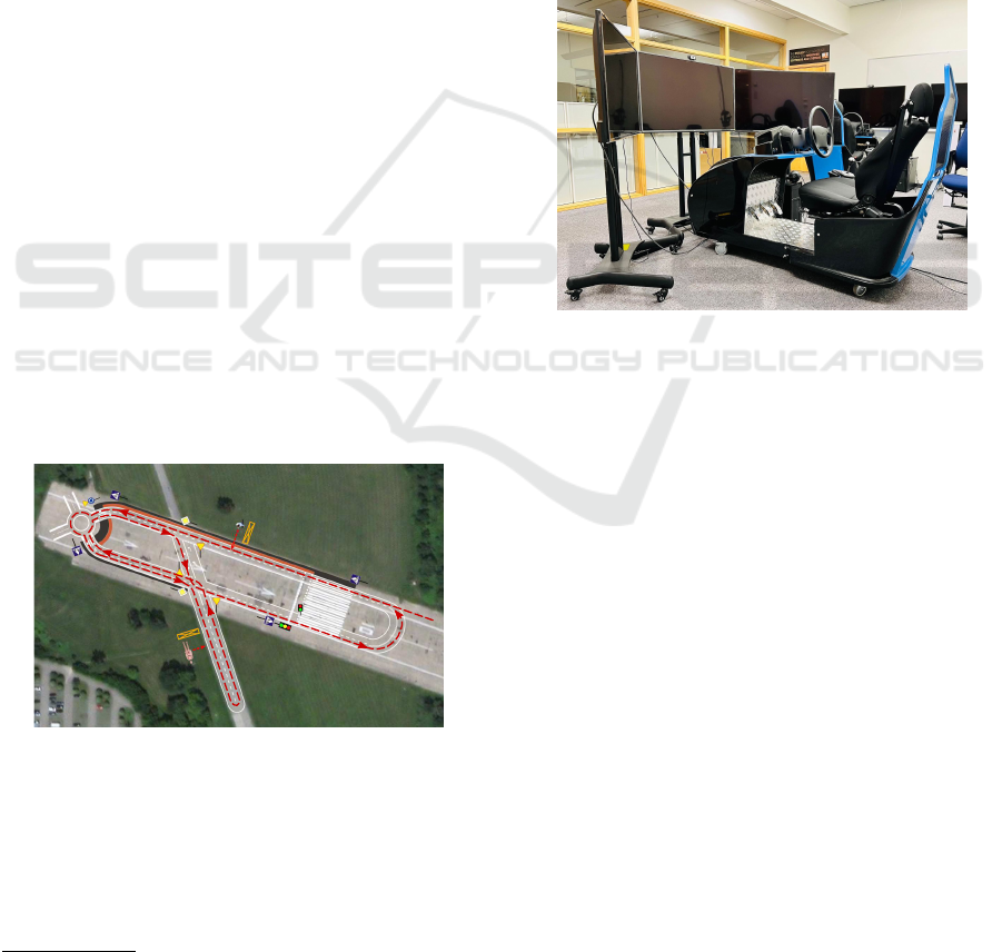
Figure 1: The experimental route for simulation and track

tests. A detailed description is presented in Section 2.1.

2.1 Experimental Protocol

The experiment to collect data for this study was con-

ducted under the framework of the European Union’s

Horizon 2020 project SIMUSAFE

(SIMUlation of

https://www.simusafe.eu/

behavioural aspects for SAFEr transport). Sixteen

drivers were recruited for participating in the study.

There were both male and female drivers. They were

selected from two age groups 18-24 and 50+ years

representing inexperienced and experienced drivers

respectively. The participants were selected in such

an order to have a homogeneous experimental group

in terms of age, sex and driving experience. The

participants were properly instructed about the ex-

periments through information meetings. Informed

consent and authorisation to use the acquired data in

the research were obtained from each participant on

paper. Throughout the experimental process, Gen-

eral Data Protection Regulation (GDPR) (Voigt and

Von dem Bussche, 2017) was strictly followed.

Figure 2: The car simulator developed with DriverSeat 650

ST was used for conducting the simulation tests.

The experimental protocol was outlined in accor-

dance with the aim of the project SIMUSAFE; to im-

prove driving simulator and trafﬁc simulation tech-

nology to safely assess risk perception and decision-

making of road users. To partially achieve the aim,

the experiment was planned with the simulator and

track driving tests. In both the simulation and track

tests, participant drivers were required to drive along

the identical route for seven laps with different vari-

ables. This design further facilitated the analysis of

varying behaviour while driving on track and simula-

tion. The route of the experiment is illustrated in Fig-

ure 1. For the track test, the route was prepared with

proper road markings, signals etc. in an old airport

in Krak

ow, Poland. In simulation tests, a modiﬁed

variant of DriverSeat 650 ST (Figure 2) simulation

cockpit was used. As annotated in Figure 1, each par-

ticipant started the lap from point A, drove straight up

to the roundabout at point B, took the third exit of the

roundabout, drove up to point C to take a right turn,

drove straight up to point D then took a U-turn and

came back to point C for a left turn and then drove

through points B (roundabout), E (right turn), C (left

Interpretable Machine Learning for Modelling and Explaining Car Drivers’ Behaviour: An Exploratory Analysis on Heterogeneous Data

393

Table 1: Associated scenarios for the laps of the experimental simulator and track driving with varying driving conditions.

Lap

Environmental Variables Driver Variables

Scenario

Events Trafﬁc Habituation Hurry Frustration Surprise

Roundabout,

Left Turn,

Intersection with

no Trafﬁc Lights

Low No No No

Drive along the route.

2 Low No No No

3 High No No No

4 Yes High No No No

5 No High Yes No No

Drive along the route and ﬁn-

ish as quickly as possible.

6 Yes High Yes Yes No

7 No High No No Yes

Drive along the route.

turn) and ﬁnishes at point F after a left curve. For the

simulation test, a similar route was designed virtually

where the participants drove following the same pro-

tocol. In both tests, a participant drove through the

route for seven laps with different scenarios contain-

ing varied environmental and driver variables as out-

lined in Table 1. The scenarios associated with the

laps were designed with the consultation of psychol-

ogists and domain experts.

2.2 Data Collection

During the whole protocol, vehicular signals, physio-

logical signals, psychological data and videos were

recorded for each participant. In this study only

the vehicular and physiological signals, speciﬁcally,

EEG, have been exploited. All the data were properly

anonymized to comply with the GDPR. The data col-

lection methods and materials are brieﬂy described in

the following sections.

2.2.1 Vehicular Signal

The acquiring of the vehicular signals as numeric de-

scriptive information was done using onboard instru-

ments accessed via vehicle Controlled Area Network

(CAN) and Inertial Measurement Unit (IMU). The

signals contained information on the parameters like

vehicle speed, acceleration, steering wheel angle, ac-

celerator and brake pedal positions, Global Position-

ing System (GPS) coordinates, yaw, roll, pitch, etc.

For track tests, the signals were directly acquired from

the vehicle unit and for simulations, the measure-

ments were recorded from the simulation framework.

In both cases, the recording frequency was 15Hz.

2.2.2 Biometric Signal

During both tests, i.e., simulation and track, the bio-

metric signals in terms of EEG were recorded us-

ing the SAGA 32+ Systems

(TMSi, The Nether-

https://www.tmsi.com/products/saga-for-eeg/

lands). Sixteen EEG channels (F p1, F pz, F p2, F7,

F3, Fz, F4, F8, P7, P3, Pz, P4, P8, O1, Oz, and

O2), placed according to the 10–20 International Sys-

tem with a Brainwave EEG Head caps, were collected

with a sampling frequency of 256Hz, grounded to

the Cz site. During the experiments, raw EEG data

were recorded and afterwards digitally ﬁltered using

a band-pass ﬁlter (2 − 70Hz) in TMSi Saga Inter-

face with FieldTrip (Oostenveld et al., 2011) integra-

tion. Finally, ARTE (Automated aRTifacts handling

in EEG) (Barua et al., 2017) algorithm was used to

remove the artefacts from the band-pass ﬁltered sig-

nals. This step was necessary because the artefacts,

e.g., eyes-blinks, could affect the frequency bands

correlated to the target measurements. However, this

method allows cleaning the EEG signal without los-

ing data and without requiring additional sensors, e.g.,

electro-oculographic sensors.

Figure 3: Event extraction using GPS coordinates. Red rect-

angles mark the signiﬁcant areas of events, e.g., roundabout,

left turn, signal with pedestrian crossing etc.

2.2.3 Event Extraction

The presented work within the framework of the

SIMUSAFE project focused on risk perception, han-

dling and hurry of drivers in urban manoeuvres that

expose higher levels of risk. In risky situations, prime

ICAART 2023 - 15th International Conference on Agents and Artiﬁcial Intelligence

394

events were short-listed by experts including round-

abouts, left turns, extensive breaking/acceleration,

etc. As per the experts’ opinion, the events were de-

ﬁned based on the road infrastructure. To label the

acquired data, all the GPS coordinates were plotted

and overlaid on the experimental track to identify the

speciﬁc GPS coordinates where an event could occur.

Figure 3 illustrates the event extraction from GPS co-

ordinates using overlaid scatter plot. Considering the

GPS coordinates within the red rectangles in Figure 3

and consulting with domain experts and psychologists

the data points were complemented with correspond-

ing events. Figure 4 illustrates the recorded GPS co-

ordinates of a single lap categorised on the basis of

road infrastructure as events in different colours. The

extracted events are further discussed in Section 3.1.

Figure 4: GPS coordinates of a single lap driving colour

coded with respect to different road structures.

2.3 Dataset Preparation

The dataset for the presented work contains two sepa-

rate sets of features and two different labels, i.e., risk

and hurry. The features were extracted from the data

collected from simulation and track tests. The process

of feature extraction was performed in two folds after

the events of interest were extracted through the utili-

sation of experts’ annotation on the raw data, i.e. spe-

ciﬁc timestamps of the events’ start and end. Based on

the experts’ annotation, for both vehicular and EEG

signals, the raw data was chunked into epochs of 2

seconds using moving window with a shift of 0.125

second to preserve the condition of stationarity of the

time-series data. Firstly, the vehicular features were

extracted. In the second step, EEG features in the fre-

quency domain were extracted and synchronised with

the vehicular features on the basis of the timestamps

of data recording. Finally, the dataset is prepared by

combining the extracted features with the events and

experts’ annotated labels.

The vehicular feature sets were populated using

the signals from vehicle CAN and IMU. The major

features extracted from the vehicle CAN are speed,

accelerator pedal position and steering wheel angle.

The average and standard deviation of these measures

were were calculated within the start and end time of

the events annotated by the experts. These features

were gathered in the feature list including the max-

imum value for speed only resulting in 7 features.

From IMU, the parameters for angular and linear ac-

celeration were considered and 9 features were cal-

culated. All the features extracted from the vehicular

signals are listed in Table 2.

Table 2: List of features extracted from vehicular signals.

Feature Name Count Source

Max. Speed

07 CAN

Avg. Speed

Std. Dev. Speed

Avg. Accelerator Pedal Pos.

Std. Dev. Accelerator Pedal Pos.

Avg. Steering Angle

Std. Dev. Steering Angle

Yaw

09 IMU

Yaw Rate

Roll

Roll Rate

Pitch

Pitch Rate

Lateral Acceleration

Longitudinal Acceleration

Vertical Acceleration

Avg.- Average, Max.- Maximum, Pos.- Position,

Std. Dev.- Standard Deviation.

From the curated EEG signals, 14 frequency do-

main features were extracted from the power spec-

tral density values. At ﬁrst, the Individual Alpha Fre-

quency (IAF) (Corcoran et al., 2018) values were es-

timated as the peak of the general alpha rhythm fre-

quency (8 −12Hz). Eventually, the average frequency

of the theta band [IAF − 6, IAF − 2], alpha band

[IAF −2, IAF + 2] and beta band [IAF + 2, IAF + 18],

over all the aforementioned EEG channels were cal-

culated. Next, the channels were partitioned on the

basis of frontal and parietal locations on the scalp. For

alpha and beta bands, frontal and parietal parts were

again divided into two segments; upper and lower.

For each of the segments, the average values of the

frequency bands were considered as a feature, thus,

obtaining a total of fourteen biometric features. Table

3 presents the list of the extracted biometric features

Interpretable Machine Learning for Modelling and Explaining Car Drivers’ Behaviour: An Exploratory Analysis on Heterogeneous Data

395

that have been further deployed in classiﬁcation tasks.

Table 3: List of biometric features considering different fre-

quency bands of EEG signal.

Feature Name Count Source

Frontal Theta

14 EEG

Parietal Theta

Frontal Alpha

Lower Frontal Alpha

Upper Frontal Alpha

Parietal Alpha

Lower Parietal Alpha

Upper Parietal Alpha

Frontal Beta

Lower Frontal Beta

Upper Frontal Beta

Parietal Beta

Lower Parietal Beta

Upper Parietal Beta

Summarising, a total of 30 features were extracted

from the vehicular and biometric data recorded from

the simulation and track tests. Among those, 16 fea-

tures were extracted from the vehicle CAN & IMU

sensors and 14 features were extracted from EEG sig-

nals. In addition to the libraries mentioned in re-

spective sections, Python libraries NumPy and Pandas

were also employed for data preparation.

After the feature extraction, the data points were

clustered into various events as described in Section

2.2.3. For each event, the data point was labelled with

associated risk and hurry based on the laps of the ex-

perimental protocol (Table 1) and psychologists’ as-

sessment. Each instance was labelled with ’yes’ or

’no’ for risk and hurry depending on their presence in

the behaviour of the corresponding participant. The

procedure produced 1771 data instances with varied

numbers of instances for different labels of risk and

hurry. Initially, the dataset was found to be largely

imbalanced. To enhance the further analysis the in-

stances with minority class for both risk and hurry

were upsampled using SMOTE (Chawla et al., 2002).

Table 4 presents the summary of the dataset.

2.4 Classiﬁer and Explanation Models

This section brieﬂy describes the models invoked in

the presented work. Prior to the discussion on the

models, the utilized dataset is theoretically formu-

lated here. The data prepared as described in Section

2.3 is D comprising of feature set X and labels Y , i.e.

D = (X,Y ). Each instance x

∈ X where i = 1, ..., n,

contains features f

∈ F where j = 1, ...,m. The labels

Table 4: Summary of the datasets from the simulator and

track experiments for risk and hurry classiﬁcation. The val-

ues represent the number of instances for corresponding la-

bels of the classiﬁcation tasks before applying SMOTE.

Classiﬁcation Label

Experiment

Total

Simulation Track

Risk

Yes 330 215 545

No 696 530 1226

Hurry

Yes 201 19 220

No 825 726 1551

Total Instance 1026 745 1771

∈ Y are associated with the corresponding instance

∈ X which varies on different classiﬁcation tasks,

i.e., risk and hurry. For all the tasks, D is split into

train

and D

test

at a ratio of 80 : 20 respectively.

2.4.1 Classiﬁer Models

The intended task is to classify risk and hurry sep-

arately which sets the context towards classiﬁcation

model c(x

). In all cases, c(x

) is trained using the

instances of X

train

⊂ X to predict the labels ˆy

. The

parameter tuning of c(x

) was performed by compar-

ing the ˆy

and y

∈ Y

train

⊂ Y .

The selection of a candidate of c(x

) was

done considering the performances of modelling car

drivers’ actions using different AI/ML models with a

similar feature set from a previous work (Islam et al.,

2020). Initially, four different classiﬁers have been

tested to classify risk and hurry. The models are

namely Logistic Regression (LR), Multilayer Percep-

tron (MLP), Random Forest (RF) and Support Vector

Machine (SVM). In addition to these models, Gradi-

ent Boosted Decision Trees (GBDT) have been also

tested for the described classiﬁcation tasks. GBDT

has been introduced in this study as an ensemble

model which complements the use of different types

of AI/ML models. The training parameters for all the

models were tuned using grid search and 5-fold cross-

validation. All the corresponding parameters for the

selected models are presented in Table 5 that were

tested in the grid search. The chosen parameters for

the classiﬁers are also highlighted in the summary ta-

ble. Python Scikit Learn (Pedregosa et al., 2011) li-

brary was invoked for training, validating and testing

the classiﬁer models.

2.4.2 Explanation Models

Literature indicates feature attribution methods are

common choices for tabular data (Liu et al., 2021; Is-

lam et al., 2022). A feature attribution method can be

denoted as f that estimates the importance w of each

ICAART 2023 - 15th International Conference on Agents and Artiﬁcial Intelligence

396

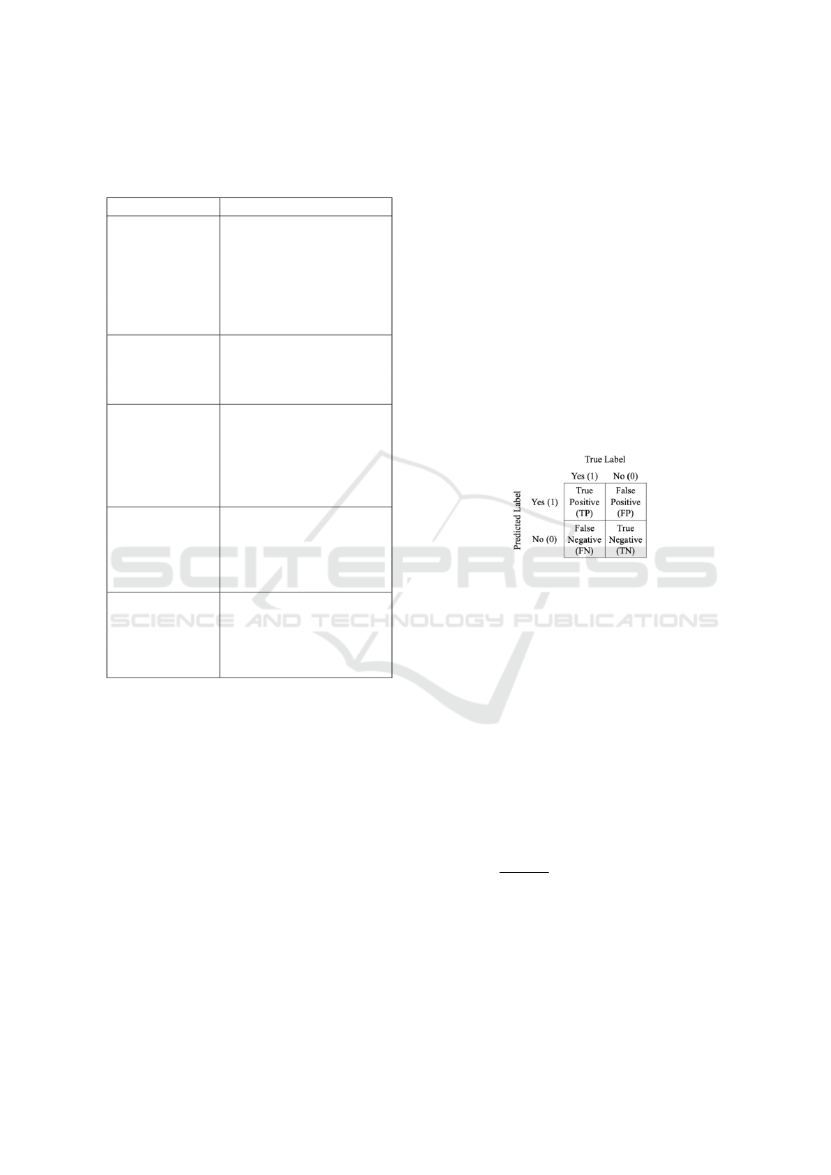
Table 5: Parameters used in tuning different AI/ML models

for classifying risk and hurry in driving behaviour with 5-

fold cross-validation. The parameters used for ﬁnal training

are highlighted in blue colour.

Classiﬁer Models Parameter Details

Gradient Boosted

Decision Trees

(GBDT)

Estimators: [100, 200, 300,

400, 500]

Learning Rate: [1e

−3

, 1e

−2

−1

, 1]

Max. Depth: [1, 3, 5, 7, 9]

Loss : [deviance,

exponential]

Logistic

Regression (LR)

C: [1e

−4

, 1e

−3

, 1e

−2

, 1e

−1

1, 1e

, 1e

]

Penalty: [l1, l2]

Solver: [liblinear]

Multilayer

Perceptron (MLP)

Hidden layers: [(32, 16, 8, 4),

(32, 16, 4), (16, 8, 4)]

Activation: [identity,

logistic, tanh, relu]

Alpha: [1e

−4

, 1e

−3

, 1e

−2

]

Solver: [adam, lb f gs, sgd]

Random Forest

(RF)

Estimators: [10, 20, 30, 40,

50, 60, 70, 80, 90, 100]

Criterion: [gini, entropy]

Max. Features: [2

, 2

]

Support Vector

Machine (SVM)

C: [1, 1e

, 1e

]

Gamma: [1e

−5

, 1e

−4

, 1e

−3

−2

, 1e

−1

, 1]

Kernel: [linear, poly, rb f ,

sigmoid]

feature to the prediction. That is, for a given classi-

ﬁer model c and a data point x

, f (c, x

) = ω ∈ R

Here, each ω

refers to the relative importance of fea-

ture j for the prediction c(x

). Among the feature

attribution methods, Shapley Additive Explanations

(SHAP) (Ribeiro et al., 2016) and Local Interpretable

Model-Agnostic Explanation (LIME) (Lundberg and

Lee, 2017) are exploited in this work as being popular

choices in present research works (Islam et al., 2022).

Both the explanation models were built for GBDT and

est to generate local and global explanations. Tree-

Explainer was invoked for SHAP to complement the

characteristics of GBDT and LIME was trained with

default settings from the corresponding library.

2.5 Evaluation

The evaluation of the presented work has been per-

formed in two folds: evaluating the performance of

the classiﬁcation models in classifying risk and hurry

in drivers’ behaviour and evaluating the feature attri-

bution using SHAP & LIME to explain the classiﬁca-

tion. The metrics used for both evaluations are brieﬂy

described in the following subsections.

2.5.1 Metrics for Classiﬁcation Model

Considering the binary classiﬁcation for both risk and

hurry, the confusion matrix (Figure 5) has been used

as the base of the evaluation of classiﬁer models, c(x).

In both the classiﬁcation tasks, the presence of risk or

hurry is considered as the positive label and absence is

considered as the negative label. In the confusion ma-

trix, True Positive (TP) and False Negative (FN) are

the numbers of correct and wrong predictions respec-

tively for the positive class, i.e., Yes (1). On the other

hand, False Positive (FP) and True Negative (TN) are

the numbers of wrong and correct predictions respec-

tively for the negative class, i.e., No (0).

Figure 5: Confusion Matrix for both Risk and Hurry Clas-

siﬁcation.

As described in Section 2.3 the dataset was pre-

pared as a balanced dataset. Considering this, the

metrics to evaluate the performance of c(x) are se-

lected to be Accuracy, Precision, Recall and F

score

as prescribed (Sokolova and Lapalme, 2009).

2.5.2 Metrics for Explanation Model

The performances of the explanation models were

measured using three different metrics; accuracy,

Normalized Discounted Cumulative Gain (nDCG)

score (Busa-Fekete et al., 2012) and Spearman’s rank

correlation coefﬁcient (ρ) (Zar, 1972).

The accuracy scores for the explanation models

were computed as the percentage of local prediction

by the explanation model that matches the classiﬁer

model, i.e.,

|c(x)≡ f(x)|

test

. This metric would reﬂect how

close the explanation models mimic the prediction of

the classiﬁer models.

To assess the feature attribution, the order of im-

portant features from the explanation models and

GBDT were considered to calculate the nDCG score

and ρ. Both measures are used to compare the or-

der of retrieved documents in information retrieval.

Speciﬁcally, nDCG score produces a quantitative

Interpretable Machine Learning for Modelling and Explaining Car Drivers’ Behaviour: An Exploratory Analysis on Heterogeneous Data

397

measure to assess the relevance between two sets of

ranks of some entities. Here, these score values were

used to evaluate the feature ranking by the explana-

tion models in contrast with the prediction model. For

nDCG, the values were calculated separately for all

the instances together and individually which are de-

noted as nDCG

all

and nDCG

ind

respectively in Table

9. Similarly, ρ produced a similar measure to evalu-

ate the quality of two vectors of ranks which was used

in parallel to support the nDCG score. Further details

on the computation of these metrics can be found in

the respective articles (Busa-Fekete et al., 2012; Zar,

1972). In this work, the values are computed using

methods from SciPy library for Python.

3 RESULTS AND DISCUSSION

The outcome of the performed analysis, classiﬁcation

tasks and explanation generation have been presented

and discussed in this section with tables and illustra-

tions. The illustrations were prepared by adopting dif-

ferent methods of the Matplotlib library of Python.

3.1 Exploratory Analysis

Aligning with the focus of project SIMUSAFE, i.e.

enhancing the simulation technologies to make the

trafﬁc environment safer, the exploratory analysis was

conducted. The outcome of the analysis was further

utilised to develop training simulators for road users

with more intelligent agents which is out of the scope

of the work presented in this paper. Though, the in-

sights explored from the analysis were used to create

intuition on the classiﬁcation tasks and explanation.

Figure 6: Average driving velocity in different laps. The

two-sided Wilcoxon signed-rank test demonstrates a sig-

niﬁcant difference in the simulator and track driving with

t = 0.0, p = 0.0156.

The ﬁrst step of the analysis was performed to as-

sess the variation of vehicular features between the

simulation and track datasets over the laps that repre-

sent different road scenarios, interchangeably termed

as events as described in Table 1. Mostly, mean values

were compared and two-sided Wilcoxon signed-rank

tests (Wilcoxon, 1992) were performed. In the sig-

niﬁcance test, the null hypothesis, H

was considered

as “there is no difference between the observations

of the two measurements”. Subsequently the alter-

nate hypothesis, H

was derived as “the observations

of the two measurements are not equal” and the level

of signiﬁcance was set to 0.05. The ﬁrst comparison

was done on the driving velocity. Figure 6 illustrates

the average driving velocity in different laps for sim-

ulation and track driving. The standard deviations are

also associated with the respective error bars in the

plot. For both tests, it was observed that average ve-

locity increased in laps 5 - 7. This aligned with the

experimental protocol. From the two-sided Wilcoxon

signed-rank test, a statistically signiﬁcant difference

was observed between simulation and track driving

(t = 0.0, p = 0.0156), thus the alternate hypothesis H

was accepted. The analysis on the accelerator pedal

position (Figure 7) produced a similar trend across

the laps for both the tests and the statistical test had

identical outcomes.

Figure 7: Average accelerator pedal position across all the

laps and the two-sided Wilcoxon signed-rank test demon-

strate a signiﬁcant difference in the simulator and track driv-

ing with t = 0.0, p = 0.0156.

From both the analysis of driving velocity and ac-

celerator pedal position, it was evident that drivers

tend to drive at a higher velocity and press the acceler-

ator pedal more in simulation tests than in track tests.

This is plausibly the cause of simulator bias. In naive

terms, drivers do not experience the motion of the

vehicle, and perceive the environment properly, e.g,

the vibration of the vehicle, the effect of road struc-

tures, etc. The differences in the driving behaviour

have been properly addressed with corresponding ex-

perts and it is a work in progress to reduce the sim-

ulation biases in future studies. Moreover, while de-

ICAART 2023 - 15th International Conference on Agents and Artiﬁcial Intelligence

398

(a) Lap 1. (b) Lap 2. (c) Lap 3.

(d) Lap 4. (e) Lap 5. (f) Lap 6.

Figure 8: GPS coordinates with varying driving velocity for a random participant in laps 1 - 6.

ploying ML algorithms to classify drivers’ behaviour,

these characteristics from non-stationary spatiotem-

poral data might lead to incorrect interpretations. To

correctly assess the effects or contribution of the het-

erogeneous features, two different methods of XAI

were evaluated and presented in Section 3.3.

The driving velocity in each lap was also anal-

ysed based on different road structures using scat-

ter plots and heatmaps as illustrated in Figure 8. In

this analysis, the seventh lap was excluded because

of the presence of surprise which reduced the data

from driving the full lap. The pattern of driving ve-

locity in laps 1 - 3 (Figure 8a - 8c) was found to be

identical. The variation increased in laps 4 - 6 (Fig-

ure 8d - 8f) when several variables were added to the

lap scenarios. The illustrated driving patterns were

cross-checked with psychologists’ assessments of the

participants and their conclusive drivers’ rules of be-

haviour. For example, on a left turn, the behaviour of

drivers can be stated as - ’if the road is one carriage-

way, then you have to gradually move on the left and

look for cars coming from the opposite direction be-

fore turning left’. In all the sub-ﬁgures of Figure 8,

it can be observed that, at the left turn near longitude

500 and latitude 750, the driver slowed down to exam-

ine oncoming vehicles and moved towards left before

the turn as to road was single carriageway by design.

Another major observation can be found in lap 6 at

the lower middle of the circuit near longitude 550 and

latitude 725 (Figure 8f). There was a signal with a

pedestrian crossing and the driving velocity was close

to zero which indicates that the stop signal was lit or

a pedestrian was crossing and the driver responded

to the signal. Thus, drivers’ behaviours at different

events in terms of road infrastructures were analysed

and the observations were put forward to respective

experts for enhancing the quality of the agents in fu-

ture simulators.

3.2 Classiﬁcation

The classiﬁcation of drivers’ behaviour was done in

two folds; risk and hurry. It is arguable that hurried

driving can induce risk. On the contrary, hurried-

ness is often observed among drivers who drive safely.

Driving safely refers to speciﬁc behaviours as an ex-

ample is stated in Section 3.1. Based on the drivers’

rules of behaviour proposed by the experts, classi-

fying risk and hurry are considered separate tasks.

The performance of the trained models on the holdout

datasets for risk and hurry classiﬁcation are presented

in Tables 6 and 7 respectively. In both tasks appar-

ently, GBDT excelled over other models. However,

for all the datasets in both tasks, simpler ones among

the investigated models produced better performance.

The use of precision and recall was justiﬁed by the na-

ture of the classiﬁcation tasks which mostly concen-

trate the measures on classifying the positive class. In

this work, the positive class was set to be the pres-

ence of risk and hurry in drivers’ behaviour which is

more important than classifying their absence. One

notable behaviour was observed for RF that it per-

formed poorly when used on the simulation and track

dataset separately but on the combined dataset it pro-

duced the result for risk classiﬁcation. In the case of

hurry classiﬁcation, the behaviour was quite altered.

Interpretable Machine Learning for Modelling and Explaining Car Drivers’ Behaviour: An Exploratory Analysis on Heterogeneous Data

399

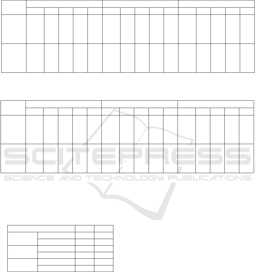
Table 6: Performance measures of risky behaviour classiﬁcation with the AI/ML models trained on the holdout test set of

different datasets. The best values for each metric and each dataset are highlighted in blue colour. (Positive Class - Risk,

Negative Class - No Risk).

Metrics

Simulation Dataset Track Dataset Combined Dataset

GBDT LR MLP RF SVM GBDT LR MLP RF SVM GBDT LR MLP RF SVM

TP 105 82 86 23 100 106 88 103 56 105 229 186 226 233 228

FN 15 38 34 97 20 0 18 3 50 1 8 51 11 4 9

FP 16 26 42 0 14 3 24 5 0 4 30 62 45 26 23

TN 112 102 86 128 114 109 88 107 112 108 199 167 184 203 206

Precision 0.868 0.759 0.672 1.0 0.877 0.972 0.786 0.954 1.0 0.963 0.884 0.75 0.834 0.900 0.908

Recall 0.875 0.683 0.717 0.192 0.833 1.0 0.830 0.972 0.528 0.991 0.966 0.785 0.954 0.983 0.962

score 0.871 0.719 0.694 0.322 0.855 0.986 0.807 0.963 0.691 0.977 0.923 0.767 0.89 0.940 0.934

Accuracy 87.50 74.19 69.36 60.89 86.29 98.62 80.73 96.33 77.06 97.71 91.85 75.75 87.98 93.56 93.13

Table 7: Performance measures of hurry classiﬁcation with the AI/ML models trained on the holdout test set of different

datasets. The best values for each metric and each dataset are highlighted in blue colour. (Positive Class - Hurry, Negative

Class - No Hurry).

Metrics

Simulation Dataset Track Dataset Combined Dataset

GBDT LR MLP RF SVM GBDT LR MLP RF SVM GBDT LR MLP RF SVM

TP 92 90 61 110 84 70 66 56 81 68 145 130 137 143 149

FN 18 20 49 0 26 11 15 25 0 13 25 40 33 27 21

FP 8 22 25 90 10 13 25 18 59 9 24 75 41 31 33

TN 91 77 74 9 89 65 53 60 19 69 174 123 157 167 165

Precision 0.920 0.804 0.709 0.550 0.894 0.843 0.725 0.757 0.579 0.883 0.858 0.634 0.770 0.822 0.819

Recall 0.836 0.818 0.555 1.0 0.764 0.864 0.815 0.691 1.0 0.840 0.853 0.765 0.806 0.841 0.876

score 0.876 0.811 0.622 0.710 0.824 0.854 0.767 0.723 0.733 0.861 0.855 0.693 0.787 0.831 0.847

Accuracy 87.56 79.90 64.59 56.94 82.78 84.91 74.84 72.96 62.89 86.16 86.69 68.75 79.89 84.23 85.33

Due to this ﬂuctuation in the performance across dif-

ferent datasets and tasks, RF was not further utilized

to develop the explanation models.

Table 8: Summary of model performances in terms of accu-

racy across different datasets and classiﬁcation tasks.

Dataset Risk Hurry

Simulation

Model GBDT GBDT

Accuracy (%) 87.50 87.56

Track

Model GBDT SVM

Accuracy (%) 98.62 86.16

Combined

Model RF GBDT

Accuracy (%) 93.56 86.69

Table 8 presents the best classiﬁer for both risk

and hurry classiﬁcation across the three datasets. It is

observed that overall GBDT performed better in ev-

ery combination that lead to its use in the explanation

generation. Moreover, to accumulate all the charac-

teristics of the data in the explanation model only the

combined dataset has been used further.

3.3 Explanation

Considering the prediction performance of GBDT

across datasets and classiﬁcation tasks, explanation

models SHAP and LIME were built to explain indi-

vidual predictions, i.e, local explanations. While ex-

plaining a single instance of prediction from c both

models mimic the inference mechanism of c to predict

the instance within their framework. The prediction

performance of the explanation model was measured

with local accuracy described in Section 2.5.2 and the

values are presented in Table 9. It was observed that

for both classiﬁcation tasks, SHAP achieved higher

accuracy than LIME. Moreover, LIME performed

very poorly in local predictions for risk classiﬁcation.

However, both explanation models performed com-

paratively poorer in terms of hurry classiﬁcation.

It is arguably presented in the literature that the

feature importance value of a feature from a classi-

ﬁer is different in terms of weights from the contri-

bution of the feature in an additive feature attribution

model (Letzgus et al., 2022). However, normalizing

the feature importance from GBDT and the contribu-

ICAART 2023 - 15th International Conference on Agents and Artiﬁcial Intelligence

400

Order

GBDT SHAP LIME

14 15 15

9 10 14

20 22 24

6 9 25

13 24 30

15 20 21

10 6 9

8 16 20

3 2 5

21 19 19

12 27 28

1 1 1

7 4 6

19 17 13

11 18 12

4 7 11

22 8 8

18 11 7

28 29 27

17 13 4

24 21 18

27 30 29

30 26 23

29 23 16

23 28 26

2 5 2

5 3 3

16 12 10

25 14 22

26 25 17

Order

GBDT SHAP LIME

15 9 9

17 21 25

22 20 17

13 11 10

25 22 26

14 25 24

6 24 21

7 10 29

11 7 20

2 8 6

10 6 4

9 4 3

3 3 8

1 1 1

18 26 14

16 23 13

8 18 23

19 14 5

20 13 12

12 15 16

27 19 19

23 28 22

28 16 7

30 29 30

26 17 15

5 5 11

21 12 18

4 2 2

24 27 27

29 30 28

Figure 9: Feature importance values are extracted from GBDT, SHAP & LIME, normalized and illustrated with horizontal bar

charts for corresponding classiﬁcation tasks. The order of the features based on the importance values is presented in tables

on either side. Features with the same order across methods are highlighted in the order tables.

Figure 10: Low ﬁdelity prototype of proposed drivers’ behaviour monitoring system for simulated driving.

tions from SHAP and LIME produced several simi-

larities in the chosen order of features by the meth-

ods. For example, all three methods had the same

feature as the most inﬂuential one in both tasks; ver-

tical acceleration for risk and standard deviation of

accelerator pedal position in hurry classiﬁcation (Fig-

Interpretable Machine Learning for Modelling and Explaining Car Drivers’ Behaviour: An Exploratory Analysis on Heterogeneous Data

401

Table 9: Pairwise comparison of performance metrics for

SHAP and LIME on combined X

test

(holdout test set) for

risk and hurry. For all the metrics, higher values are bet-

ter and highlighted in blue colour. All the values for ρ are

statistically signiﬁcant since P < 0.05.

Metrics

Risk Hurry

SHAP LIME SHAP LIME

Accuracy 92.59% 52.98% 84.32% 70.06%

0.9561 0.8758 0.9588 0.9183

0.8717 0.8589 0.8671 0.8524

ρ, P

0.7664, 0.5310, 0.7059, 0.4772,

7.91e

−7

2.53e

−3

1.31e

−5

7.67e

−3

ure 9). In risk classiﬁcation, it is justiﬁed that vertical

acceleration is the most contributing feature as it cor-

responds to the lifting of the front part of the vehicle

due to sudden acceleration. In this scenario, the vehi-

cle often gets out of control and the concerned events

are - driving at the roundabout exits with pedestrian

crossing, manoeuvring after a left turn, etc. In the

other classiﬁcation task for hurry, the standard devia-

tion of the accelerator pedal position corresponds to a

frequent pressing of the pedal with a varying intensity

which is plausibly an indication to hurry. Here, the

concerned events are similar to the events mentioned

for risk.

Several similar ranks of the features based on their

contributions from both SHAP and LIME motivated

the comparison of nDCG scores that computes the

similarity of retrieved information. In this work, the

retrieved information is the order of features accord-

ing to their importance values or contributions to pre-

diction. The nDCG scores were computed for all the

instances together and also computed for individual

predictions and averaged. The rank of the features

based on the normalized feature importance from the

base model GBDT was used as the reference while

calculating the nDCG score to assess how similar

they are to the classiﬁer model. Alike local accuracy,

SHAP produced better results than LIME in terms of

nDCG score. To investigate further, ρ was computed

with a null hypothesis, ’the rank of the features in dif-

ferent methods are different’. However, with the test

results, the hypothesis was rejected as all the measure-

ments came out to be statistically signiﬁcant as the P

value was lower than 0.05. All the values of nDCG

score and ρ are reported in Table 9. Another notewor-

thy aspect was observed from the metrics evaluating

the explanation models that SHAP produced better

results for risk classiﬁcation but the performance of

LIME was better for hurry classiﬁcation. The perfor-

mance of SHAP complements the performance sum-

mary of the classiﬁcation models presented in Table 8

where risk classiﬁcation had better performance than

hurry classiﬁcation. It is also plausible that, if the

local accuracy of an explanation model is better, the

rankings of the attributed features are also more rel-

evant which is evident in the corresponding nDCG

score and ρ values.

3.4 Proposed Interpretable System

Combining all the presented outcomes, a proposed

system is designed for drivers’ behaviour monitoring

for simulated driving. Figure 10 illustrates a low-

ﬁdelity prototype of the proposed system. The pro-

totype consists of three segments; A, B and C which

also represent the ﬂow of operation of the system. In

segment A, a list of participants and their driven laps

will be listed. Upon selecting a participant and spe-

ciﬁc lap, the GPS plot of the lap will be presented in

segment B with a heatmap representing the driving

velocity. Moreover, the events in terms of road in-

frastructure will be marked in green rectangles. The

event rectangles will be coloured red and orange for

the presence of risk and hurry respectively. For con-

current presence, there will be a double rectangle as

shown in the illustration. In the next step, if an event

with risk or hurry is clicked, segment C will present

the contributing features to the speciﬁc classiﬁcation

and their contributions in terms of SHAP values. In

the prototype, an explanation for the selected risky

event is shown. For segment C, users can also set the

number of contributing features to display in the top

right corner. This system can be efﬁciently utilized

to analyse drivers’ behaviour to correct driving styles

to ensure a safer road environment for all users. The

information shown in segment C contains the features

from both vehicle and EEG which are relevant to the

risky and hurried behaviour of the drivers according to

the literature. An expert from the corresponding do-

main can relate the change in feature values and their

effect on the prediction and convey speciﬁc instruc-

tions to modify the drivers’ behaviour to make their

driving safer.

4 CONCLUSIONS AND FUTURE

WORKS

The work presented in this paper can be summarised

in three aspects: i) comparative analysis of car

drivers’ behaviour in the simulator and track driving

for different trafﬁc situations, ii) development of clas-

siﬁer models to detect risk or hurry in drivers’ be-

haviour and iii) explaining the risk and hurry clas-

siﬁcation with feature attribution techniques with a

proposed system for drivers’ behaviour monitoring in

simulated driving. The ﬁrst outcome is found to be

ICAART 2023 - 15th International Conference on Agents and Artiﬁcial Intelligence

402

a novel analysis that includes experimentation with

simulation and track driving. The second and third

outcomes can be concurrently utilised in enhancing

the simulator techniques to train road users for a safer

trafﬁc environment through the functional develop-

ment of the proposed drivers’ behaviour monitoring

system.

The outcome of this study is encouraging in terms

of explanation methods that require further research.

The lack of prescribed evaluation metrics in the lit-

erature led to the use of different borrowed metrics

from different concepts. However, the results showed

promising possibilities to enhance and modify them

for future works on the evaluation of explanation

methods. Another possible research direction would

be to improve the feature attribution methods to pro-

duce more insightful explanations.

ACKNOWLEDGEMENTS

This study was performed as a part of the project

SIMUSAFE funded by the European Union’s Hori-

zon 2020 research and innovation programme under

grant agreement N. 723386.

REFERENCES

Abadi, M. L. and Boubezoul, A. (2021). Deep neural net-

works for classiﬁcation of riding patterns: with a focus

on explainability. In Proceedings of the 29th Euro-

pean Symposium on Artiﬁcial Neural Networks, Com-

putational Intelligence and Machine Learning.

Antwarg, L., Miller, R. M., Shapira, B., and Rokach, L.

(2021). Explaining anomalies detected by autoen-

coders using shapley additive explanations. Expert

Systems with Applications, 186:115736.

Barua, S., Ahmed, M. U., Ahlstrom, C., Begum, S., and

Funk, P. (2017). Automated EEG Artifact Handling

with Application in Driver Monitoring. IEEE Journal

of Biomedical and Health Informatics, 22(5):1350.

Busa-Fekete, R., Szarvas, G., Elteto, T., and K

egl, B.

(2012). An Apple-to-Apple Comparison of Learning-

to-Rank Algorithms in terms of Normalized Dis-

counted Cumulative Gain. In ECAI 2012-20th Euro-

pean Conference on Artiﬁcial Intelligence: Preference

Learning: Problems and Applications in AI Work-

shop, volume 242. Ios Press.

Chawla, N. V., Bowyer, K. W., Hall, L. O., and Kegelmeyer,

W. P. (2002). SMOTE: Synthetic Minority Over-

Sampling Technique. Journal of Artiﬁcial Intelligence

Research, 16:321–357.

Corcoran, A. W., Alday, P. M., Schlesewsky, M., and

Bornkessel-Schlesewsky, I. (2018). Toward a Re-

liable, Automated Method of Individual Alpha Fre-

quency Quantiﬁcation. Psychophysiology, 55(7).

Islam, M. R., Ahmed, M. U., Barua, S., and Begum, S.

(2022). A Systematic Review of Explainable Artiﬁ-

cial Intelligence in terms of Different Application Do-

mains and Tasks. Applied Sciences, 12(3):1353.

Islam, M. R., Barua, S., Ahmed, M. U., Begum, S., Aric

P., Borghini, G., and Di Flumeri, G. (2020). A Novel

Mutual Information based Feature Set for Drivers’

Mental Workload Evaluation using Machine Learn-

ing. Brain Sciences, 10(8):551.

Letzgus, S., Wagner, P., Lederer, J., Samek, W., M

uller,

K.-R., and Montavon, G. (2022). Toward Explain-

able Artiﬁcial Intelligence for Regression Models: A

Methodological Perspective. IEEE Signal Processing

Magazine, 39(4):40–58.

Liu, Y., Khandagale, S., White, C., and Neiswanger, W.

(2021). Synthetic benchmarks for scientiﬁc research

in explainable machine learning. arXiv preprint

arXiv:2106.12543.

Lundberg, S. M. and Lee, S.-I. (2017). A Uniﬁed Approach

to Interpreting Model Predictions. Advances in neural

information processing systems, 30.

Oostenveld, R., Fries, P., Maris, E., and Schoffelen, J.-M.

(2011). FieldTrip: Open Source Software for Ad-

vanced Analysis of MEG, EEG, and Invasive Electro-

physiological Data. Computational Intelligence and

Neuroscience, 2011.

Pedregosa, F., Varoquaux, G., Gramfort, A., Michel, V.,

Thirion, B., Grisel, O., Blondel, M., Prettenhofer, P.,

Weiss, R., and Dubourg, V. (2011). Scikit-learn: Ma-

chine Learning in Python. The Journal of Machine

Learning Research, 12:2825–2830.

Ribeiro, M. T., Singh, S., and Guestrin, C. (2016). ”Why

should I trust you?” Explaining the Predictions of any

Classiﬁer. In Proceedings of the 22nd ACM SIGKDD

international conference on knowledge discovery and

data mining, pages 1135–1144.

Sætren, G. B., Lindheim, C., Skogstad, M. R., Andreas Ped-

ersen, P., Robertsen, R., Lødemel, S., and Haukeberg,

P. J. (2019). Simulator versus Traditional Training: A

Comparative Study of Night Driving Training. In Pro-

ceedings of the Human Factors and Ergonomics So-

ciety Annual Meeting, volume 63, pages 1669–1673.

SAGE Publications Sage CA: Los Angeles, CA.

Serradilla, O., Zugasti, E., Ramirez de Okariz, J., Ro-

driguez, J., and Zurutuza, U. (2021). Adaptable and

explainable predictive maintenance: semi-supervised

deep learning for anomaly detection and diagnosis in

press machine data. Applied Sciences, 11(16):7376.

Sokolova, M. and Lapalme, G. (2009). A Systematic Analy-

sis of Performance Measures for Classiﬁcation Tasks.

Information processing & management, 45(4):427.

Voigt, P. and Von dem Bussche, A. (2017). The EU Gen-

eral Data Protection Regulation (GDPR). A Practical

Guide, 1st Ed., Cham: Springer International Pub-

lishing, 10:3152676.

Wilcoxon, F. (1992). Individual Comparisons by Ranking

Methods. In Breakthroughs in statistics, pages 196–

202. Springer.

Wu, S.-L., Tung, H.-Y., and Hsu, Y.-L. (2020). Deep

Learning for Automatic Quality Grading of Mangoes:

Interpretable Machine Learning for Modelling and Explaining Car Drivers’ Behaviour: An Exploratory Analysis on Heterogeneous Data

403

Methods and Insights. In 2020 19th IEEE Interna-

tional Conference on Machine Learning and Applica-

tions (ICMLA), Miami, FL, USA. IEEE.

Zar, J. H. (1972). Signiﬁcance Testing of the Spearman

Rank Correlation Coefﬁcient. Journal of the American

Statistical Association, 67(339):578–580.

Zhou, F., Alsaid, A., Blommer, M., Curry, R., Swami-

nathan, R., Kochhar, D., Talamonti, W., and Tije-

rina, L. (2021). Predicting Driver Fatigue in Auto-

mated Driving with Explainability. arXiv preprint

arXiv:2103.02162.

ICAART 2023 - 15th International Conference on Agents and Artiﬁcial Intelligence

404