Optimization of Direct Transportation Flows for the Removal of
Construction Waste Bins with both Resource and Task Availability
Interval Constraints
Safae Abderebbi and Wahiba Ramdane Cherif-Khettaf
a
LORIA, UMR 7503, Mines Nancy, Lorraine University, Nancy, France
Keywords: Waste Transportation, Waste Bin Removal, Parallel Machine Scheduling Problem, Multiple Availability
Interval Constraints, Mixed Integer Programming.
Abstract: This study focuses on a new real-word problem encountered in the construction sector, which concerns the
optimization of the removal of construction waste bins from construction sites to a massification platform,
where a limited heterogeneous fleet of tipper trucks (vehicles) must perform direct trips from the platform to
the construction sites to collect the waste bins. Each vehicle has a capacity of one bin, it leaves the platform
with an empty bin, travels to the construction site, drops off the empty bin in the construction site, collects
the full bin and returns to the platform to unload the full bin. The issue is that the vehicles and the construction
sites have one or more periods of availability, and thus are not available any time. This problem is modeled
as a parallel machine scheduling problem of bin removal tasks on non-identical machines (vehicles), with
new constraints that concern the presence of multiple availability intervals for both vehicles and tasks. Two
mixed-integer programming (MIP) models are presented and evaluated on 18 new instances derived from real
industrial case study.
1 INTRODUCTION
As the construction industry develops, it generates an
enormous quantity of materials and a very large
quantity of waste. In France
1
, the construction sector
is responsible for almost 45% of national energy
consumption, over 25% of greenhouse gas emissions,
and generates over 42 million tons of waste per year.
Legislation in France proposes a more global
approach to the environmental impact of the
construction sector including a better management of
the construction supply chain. Thus, sorting,
recycling and valorization of construction waste has
become important for improving the environmental
and ecological performance of the construction
industry. This issue is studied in the French
framework of the R&D project DILC which refers to
“demonstrator innovations logistic sites”, whose aim
is to design an innovative platform for optimizing
construction site logistics, that is adapted to multi-site
a
https://orcid.org/0000-0002-2822-0262
1
https://www.optigede.ademe.fr/outils-multi-acteurs/ba
timents-et-travaux-publics/dechets-du-batiment/cadre-
reglementaire
ecocity construction projects. The DILC project
focuses on the consolidation of transport flows and
human resources through a physical platform that is
modular, removable, and mobile, and the
development of decision support tools to help the
platform managers to optimize their logistics.
The platform must also manage the removal of
waste from construction sites to the platform. The
platform offers a recycling area to sort and recycle the
collected waste, and a material shop for the reuse of
some of this waste. Better management of waste
transport flows from the sites to the platform will
permit to extend the ecological efforts of the building
sector to the construction phase. It should be noted
that there are two types of waste: Big-bag waste and
waste bin. Big-bag wastes are packed on pallets and
concern wastes that are produced with small and
medium quantities such as soft plastic, hard plastic,
and cardboard. Waste bin concerned the wastes that
are produced in large quantity like wood and metals.
Abderebbi, S. and Ramdane Cherif-Khettaf, W.
Optimization of Direct Transportation Flows for the Removal of Construction Waste Bins with both Resource and Task Availability Interval Constraints.
DOI: 10.5220/0011821900003396
In Proceedings of the 12th International Conference on Operations Research and Enterprise Systems (ICORES 2023), pages 221-228
ISBN: 978-989-758-627-9; ISSN: 2184-4372
Copyright
c
 2023 by SCITEPRESS – Science and Technology Publications, Lda. Under CC license (CC BY-NC-ND 4.0)
221

The optimization of the Big-bag removal is studied in
(Jaballah and Ramdane Cherif-Khettaf, 2021;
Ramdane Cherif-Khettaf et al., 2022) where a new
vehicle routing model called the Multi-Trip Pickup
and Delivery Problem, with Split loads, Profits and
Multiple Time Windows was proposed. This model
allowed mutualization of material delivery with Big-
Bag waste removal, using tail-lift truck fleet. In this
study, we focus only on waste bin removal, which
consists in performing a set of direct trips from the
platform to the construction sites to satisfy
construction site requests for full bins removal and
their replacement by empty bins. The remainder of
the paper is organized as follows. Section 2 describes
the problem and related literature; two MIP models
are presented in section 3. Experimental results with
the definition of benchmarks are given in section 4.
Finally, concluding remarks are given in section 5.
2 PROBLEM DESCRIPTION AND
RELATED LITERATURE
A limited heterogeneous fleet of tipper trucks
(vehicles) situated at the platform must perform
multiple direct trips between the platform and the
construction sites. The vehicles differ by their speed
and their distance limit. Each trip consists of loading
an empty bin at the platform, delivering it to a given
construction site, collecting a full waste bin from this
construction site, and unloading it in the recycling
center located just next to the platform. Each vehicle
has one or more periods of availability, which
represent the time windows when the vehicles are
available at the platform and so can move to the
construction sites to collect waste bins, outside of
these periods of availability, the vehicles can be
mobilized for other tasks external to the platform and
can’t satisfy the request of bin removal. The platform
also has a period of availability, that is given by the
platform's opening hours. The construction sites have
one or more types of bins depending on the specificity
of the works in progress in the construction site (bin
for wood, bin for metals, bin for plaster, bin for inert
materials, etc.). Each site has only one bin per type,
and must therefore send to the platform requests for
bin removal. The platform must manage the bins
waste removal with the available resources and
ensure the replacement of each full bin with an empty
one. The construction sites also have one or more
periods of availability during which vehicles access is
allowed, and thus the arrival and departure of vehicles
at the construction site location must be within one of
the availability time windows allowed by the
construction site. We denote by a bin removal task,
all operations that consists of loading the vehicle with
an empty bin at the platform, travelling from the
platform to the construction site, unloading the empty
bin at the construction site, loading the full bin,
travelling back to the platform and unloading the full
bin at the platform's recycling center. Platform
service time is the time required for loading and
unloading the bin on the platform.
This problem can be modelled as unrelated
parallel machine scheduling problem in which the
vehicles can be represented as machines with multiple
periods of availability and the bin removal tasks as
jobs that have one or multiple periods of availability,
and require a certain amount of processing time, that
depends on the vehicle that is used. In addition, the
constraint of availability of the tasks in our case
concerns only a part of the task processing time, it is
the loading and unloading part at the location of the
construction site and does not concern the part of the
travel to and from the site. The objective is to perform
the maximum number of bin removal tasks, to
determine the assignment of tasks to the availability
intervals of the vehicles; and to define the sequence
of satisfied tasks per available interval of each used
vehicle.
In terms of computational complexity (Lenstra et
al., 1977) proved that the single machine scheduling
problem with only release dates, which is a special
case of our problem is NP-hard. In literature,
extensive studies have been conducted in the area of
parallel machine scheduling with time constraints
without availability constraints (Arik et al.,2022;
Osorio-Valenzuela et al., 2019). In most of the
research reviewed in the area of parallel machine
scheduling, the availability constraints are defined on
resources (Such-Jeng, 2013). Very few studies
consider the availability intervals of tasks as in
(Gedik et al.,2016). A survey on parallel machine
scheduling under availability constraints can be found
(Kaabi and Harrath, 2014).
Despite the abundant literature on parallel
machine scheduling, the problem that we present here
is in our knowledge a novel one and allows us to
model a new constraint in unrelated parallel machine
scheduling problems, that is both resource and task
multiple availability interval constraint. Our
contribution can be summarized in the two following
issues:
─ Modeling a real problem of direct transportation
of bin waste in the construction sector as a
parallel machine scheduling problem with a new
specific constraint that is multiple periods of
ICORES 2023 - 12th International Conference on Operations Research and Enterprise Systems
222

availability of both resources and tasks. In
addition, the period of availability of tasks in our
case concerns only a part of the task processing
time, it is the loading and unloading part in the
construction site. The travel time which is a part
of the processing time is not concerned by the
task availability interval.
─ Proposing of two mixed-integer programming
(MIP) models, and analysis of results on 18
instances provided by our industrial partners.
3 NOTATION AND
MATHEMATICAL
PROGRAMMING MODELS
For a given time horizon specified by the platform's
opening time window, we seek to assign n non-
identical jobs (bin removal tasks) to K non-identical
machines (vehicles). The objective is to provide the
best sequence of bin removal tasks on each vehicle
to perform a maximum of bin removal tasks.
Moreover, the processing time of each bin removal
tasks depends on the type of vehicle that is assigned
to it. Each bin removal task has a processing time, that
includes loading and unloading time in the platform,
travel time from the platform to the construction site
and from the construction site to the platform. Note
that task service time represents only loading and
unloading at the construction site. Each task has DC
periods of availability intervals for its task service,
and each vehicle has DV periods of availability
intervals. The objective is to maximize the total
number of tasks to be performed within a given time
horizon.
We first define the parameters and decision
variables, and then present the two proposed
mathematical models.
Indices:
i, j : task index (1, . . ., n)
k : vehicle index, k = 1, . . ., K
α : task availability interval index,
α = 1,.., DC
l : vehicle availability interval index,
l = 1, . . ., DV
Parameters:
n : total number of tasks
K : total number of vehicles
DC : total number of tasks’ availability
intervals
DV : total number of vehicles’ availability
intervals
M : a very large number
CP : platform loading time
DP : platform unloading time
rp : release date of the platform’s time
window
dp : due date of the platform’s time
window
timePC
ik
: duration between the platform and the
construction site i, using vehicle k
CS
i
: site i loading time
DS
i
: site i unloading time
timeTask
ik
: processing time of task i using vehicle
k, such that:
timeTask
ik
= CP + 2 ×
timePC
ik
+CS
i
+DS
i
+DP
rs
iα
: release date of availability interval α of
task i
ds
iα
: due date of availability interval α of
task i
dist
i
: round-trip distance between the
platform and the construction site i
distmax
k
: maximum distance of each vehicle k
timeInter
kl
: duration of availability interval l of
vehicle k
rv
kl
: release date of availability interval l of
vehicle k
dv
kl
: due date of availability interval l of
vehicle k
Decision Variables
V
k
: 1, if vehicle k is used; 0, otherwise
Y
iαkl
: 1, if task i is scheduled using its
availability interval α on availability
interval l of vehicle k; 0, otherwise
Z
ij
: 1, if task i precedes task j; 0,
otherwise
T
i
: task i start time; 0 if i is not assigned
to any vehicle
3.1 Mixed Integer Programming
(MIP1)
The first mathematical model that will be referred to
as MIP1 is given below:
(MIP1) Maximize
∑∑ ∑ ∑
𝑌








iαk
(1)
St.
∑∑∑
𝑌





 
iαkl
1 , ∀𝑖 (2)
V
k
≤
∑∑ ∑
𝑌



 


iαkl
, ∀𝑘 (3)
Optimization of Direct Transportation Flows for the Removal of Construction Waste Bins with both Resource and Task Availability Interval
Constraints
223

∑∑ ∑
𝑌






iαkl
 𝑀
4
*V
k
,∀𝑘 , 𝑀
4
= n (4)
T
i
 𝐶𝑃  𝑡𝑖𝑚𝑒𝑃𝐶
ik
 𝑟𝑠
iα
𝑀
5
 
∑
𝑌


iαkl
 1
∀𝑖,𝛼,𝑘, M
5
= DP (5)
T
i
 𝐶𝑃  𝑡𝑖𝑚𝑒𝑃𝐶
ik
 𝐶𝑆
i
 𝐷𝑆
i
 𝑑𝑠
iα
𝑀
6
*
(1 
∑
𝑌


iαkl
), ∀𝑖 , α, 𝑘, M
6
= DP + timeTask
ik
(6)
T
i
𝑟𝑣
k
 𝑀
7
 
∑
𝑌


iαkl
 1, ∀𝑖, 𝑘, 𝑙, M
7
= DP
(7)
T
i
 𝑡𝑖𝑚𝑒𝑇𝑎𝑠𝑘
ik
𝑑𝑣
kl
 𝑀
8
 1 
∑
𝑌


iαkl
)
∀𝑖 , 𝑘 , l , M
8
= 1.5  DP (8)
∑∑ ∑
𝑑𝑖𝑠𝑡






i
 𝑌
iαkl
𝑑𝑖𝑠𝑡𝑚𝑎𝑥
k
 V
k
,∀𝑘
(9)
∑∑
𝑌




iαkl
 𝑡𝑖𝑚𝑒𝑇𝑎𝑠𝑘
ik
 𝑡𝑖𝑚𝑒𝐼𝑛𝑡𝑒𝑟
kl
,∀𝑘,𝑙 ) (10)
∑∑∑
𝑌





 
iαkl
 T
i
,∀𝑖 (11)
T
i
 𝑀
12

∑∑∑
𝑌






iαkl
,∀𝑖, M
12
= DP
(12)
T
i

∑
𝑌


iαkl
 timeTask
ik
)  T
j
 𝑀
13
 (3 
∑
𝑌


iαkl

∑
𝑌


jαkl
- Z
ij
),
∀𝑖 𝑗,𝑘,𝑙, M
13
= DP (13)
T
j

∑
𝑌


iαkl
 timeTask
jk
) 
T
i
 𝑀
14
 (2 
∑
𝑌


iαkl

∑
𝑌


jαkl
+ Z
ij
),
∀𝑖 𝑗,𝑘,𝑙, M
14
= DP (14)
V
k
∈

0, 1

,∀𝑘 ; 𝑌
iαkl
∈

0, 1

,∀𝑖,𝑘,𝑙,𝛼 ; 𝑍
ij
∈

0, 1

,∀𝑖,𝑗 ; T
i
 0, ∀𝑖 (15)
The objective function (1) maximizes the number
of tasks. Constraint (2) guarantees that each task is
scheduled at most once, fulfilling one task availability
interval and one vehicle availability interval.
Constraints (3) and (4) ensure the coherence between
Yiαkl and Vk . Constraints (5) and (6) state that the
start time of the task, which represents the beginning
of the loading of an empty bin at the platform must
allow the vehicle to arrive at the site i and to perform
the service on the site i (unloading the empty bin and
loading the full bin) while meeting one of the task
availability intervals. Constraint (7) and (8) guarantee
that the start time of the task must respect the release
date and the due date of one of the interval
availabilities of the vehicle that is selected. Constraint
(9) means that each vehicle must satisfy its maximum
distance. Constraint (10) ensures that the sum of the
processing times of all tasks assigned to a given
interval must satisfy the time duration of this interval.
Constraints (11) and (12) represent coherence
constraint between Ti and Yiαkl . Constraints (13)
and (14) force a precedence relation between two
tasks if they use the same vehicle availability period.
Constraints (15) are the set constraint.
3.2 Mixed Integer Programming
(MIP2)
In this section, we present another version of MIP1,
in which constraints (1)-(15) are maintained except
constraints (5) and (6) which will be reformulated in
another way:
T
i
 𝐶𝑃 
∑



𝑡𝑖𝑚𝑒𝑃𝐶
ik

∑
𝑌


iαkl
)  𝑟𝑠
iα

𝑀
5’
 
∑∑
𝑌




iαkl
 1, ∀𝑖, 𝛼, M
5’
= DP (5’)
T
i
 𝐶𝑃 
∑



𝑡𝑖𝑚𝑒𝑃𝐶
ik

∑
𝑌


iαkl
)  𝐶𝑆
i
 𝐷𝑆
i
 𝑑𝑠
iα
𝑀
6’
 1 
∑∑
𝑌




iαkl
, ∀𝑖, 𝛼,
M
6’
= DP (6’)
4 EXPERIMENTAL RESULTS
To solve our two models, we use Pyomo, an open-
source constrained optimization library and GLPK
solver. All tests were carried out on MacBookPro18,3
at 2.66 GHz, with 16 GB RAM. We conducted
numerical experiments on 18 new instances which are
inspired by real case studies given by our industrial
partners.
In this section, we give a general description of
the studied instances, we present the results that
allowed us to validate our models. We first analyze
the detailed results of the two models on an
illustrative example, then we give a comparison of the
two models and evaluate their limit on all instances.
4.1 Instance Description
The studied instances simulate a real case study
provided by our industrial partners. The number of
sites for the considered instances is 10. Each site can
have one or several requests for bin waste removal,
which gives a total number of tasks that ranges
between 10 and 20. The characteristics of the
instances are given in table 8a. Column1 indicates the
instance, this name starts with R, followed in order by
the number of sites, the instance index, the letter ‘F’
to indicate that the number of vehicles is fixed, then a
letter (U or P) means that the vehicles have only one
interval of availability (U), or multiple interval of
availability (P). The last position in the instance name
is a group number. Instances with the same group
number have the same characteristics except the total
number of tasks. i.e. the number of requests per
ICORES 2023 - 12th International Conference on Operations Research and Enterprise Systems
224

construction site is different, which results in a
different number of tasks. The two other columns
give the characteristics of each instance, which are the
following in column order: the number of sites (NS),
the number of tasks (n), the number of vehicles (K),
minimum and maximum number of availability
intervals of tasks (DC), and finally the minimum and
the maximum number of availability intervals of
vehicles (DV).
4.2 An Illustrative Example
In this section, the instance R10_1_F_P is given to
illustrate the problem environment and the solution
structure. This instance considers 10 sites, and 5
vehicles. Each site has one demand for bin removal
(1 task per site). The number of availability intervals
per site (respectively per vehicle) is between 1 and 4
(respectively between 2 and 3). All details of this
instance are given in tables 1, 2, 3, 4 and 5.
Table 1: R10_1_F_P_1 size.
K NS n [Min, Max] DC [Min, Max] DV
5 10 41 [1, 4] [2, 3]
Table 2: R10_1_F_P_1 instance - vehicle features.
V
Distmax
(km)
Speed
max
(Km/h)
DV
TimeInter
{Min(h),
Max (h)}
Intervals
V1 800 80 3 {3, 6}
[6, 12],
[14, 17],
[18, 21]
V2 600 70 2 {3,3}
[14, 17],
[18, 21]
V3 600 60 3 {3, 6}
[6, 12],
[14, 17],
[18, 21]
V4 500 50 3 {3, 6}
[6, 12],
[14, 17],
[18, 21]
V5 800 80 2 {3, 6}
[6, 12],
[14, 17]
Table 3: R10_1_F_P_1 instance - site features (DSP:
Distance between sites and the platform, the length of
intervals is equal to 1h for all sites).
Sites
DSP
(Km)
DC
CS
(h)
DS
(h)
Intervals
S1 187.24 4 0.17 0.17
[7, 8],
[11, 12],
[14, 15],
[17, 18]
S2 194.82 2 0.08 0.12
[14, 15],
[17, 18]
S3 150.26 3 0.10 0.10
[7, 8],
[14, 15],
[17, 18]
S4 32.42 2 0.13 0.10
[7, 8],
[14, 15]
S5 104.86 4 0.15 0.10
[7, 8],
[11, 12],
[14, 15],
[17, 18]
S6 140.45 2 0.17 0.17
[14, 15],
[17, 18]
S7 142.93 3 0.17 0.10
[7, 8],
[11, 12],
[14, 15]
S8 127.90 3 0.17 0.12
[11, 12],
[14, 15],
[17, 18]
S9 169.06 2 0.17 0.15
[14, 15],
[17, 18]
S10 86.62 1 0.15 0.12 [11, 12]
Table 4: R10_1_F_P_1 instance-platform features.
rp dp CP (h) DP (h)
6 21 0.10 0.13
The availability interval constraints are shown in
figure 1 for the construction site 7. We can notice for
site 7 and if we consider only vehicle 1, only the first
Optimization of Direct Transportation Flows for the Removal of Construction Waste Bins with both Resource and Task Availability Interval
Constraints
225

availability interval of site 7 can be feasible, because
the second and the third interval does not allow
vehicles to perform the travel time, when respecting
these vehicle availability intervals even if we start the
task as soon as possible (see figure 2.a and figure 2.b
for more details). If task 7 is selected in the solution,
the beginning of the service of this task will be
scheduled using the first availability interval of the
site [7h, 8h]. The task will be assigned to the
availability interval [6h, 12h] of the vehicle 1.
Table 5: R10_1_F_P_1 instance - travel time between the
platform and the sites (h).
Vehicles
Sites V1 V2 V3 V4 V5
S1 1.17 1.34 1.56 2.27 1.17
S2 1.22 1.39 2.02 2.35 1.22
S3 1.34 1.07 1.25 1.50 1.34
S4 0.20 0.23 0.27 0.32 0.20
S5 1.06 1.15 1.27 1.05 1.06
S6 1.28 1.00 1.17 1.40 1.28
S
7
1.29 1.02 1.19 1.43 1.29
S8 1.20 1.31 1.07 1.28 1.20
S9 1.06 1.21 1.41 2.09 1.06
S10 0.54 1.02 1.12 1.27 1.54
Figure 1: R10_1_F_P_1 instance – illustration of the
availability interval constraints on task 7.
Table 6: R10_1_F_P_1 – comparison between MIP1 and
MIP2.
Model Obj K
Time
(min)
MIP1 6 4 3
MIP2 6 4 1.3
The results obtained for instance R10_1_F_P by
model 1 (respectively model 2) are illustrated by a
Gantt chart in figure 3 (respectively in figure 4). The
results show that an optimal solution was found by
both models. 6 tasks were scheduled among the 10
tasks using 4 vehicles among the 5 available. Vehicle
2 is not used in both solutions, because none of the
remaining tasks is compatible with the availability
intervals of this vehicle. The two solutions one
interval for each selected vehicle except for vehicle 1
and vehicle 3, where a second interval was chosen
only for vehicle 1 in the first solution and only for
vehicle 3 in the second solution. The other selected
intervals are the same for each vehicle in the two
solutions. The tasks that have not been assigned in the
optimal solution are tasks 2, 6, 8 and 9. We can notice
that the availability intervals of these tasks are
incompatible with all the remaining availability
intervals of the vehicles.
Figure 2a: R10_1_F_P_1 - compatibility of availability
intervals [7h, 8h] and [11h, 12h] of task 7.
Figure 2b: R10_1_F_P_1- compatibility of availability
interval
[14h, 15h] of task 7.
Figure 3: R10_1_F_P_1 - Gantt chart of the optimal
solution obtained by MIP1.
ICORES 2023 - 12th International Conference on Operations Research and Enterprise Systems
226

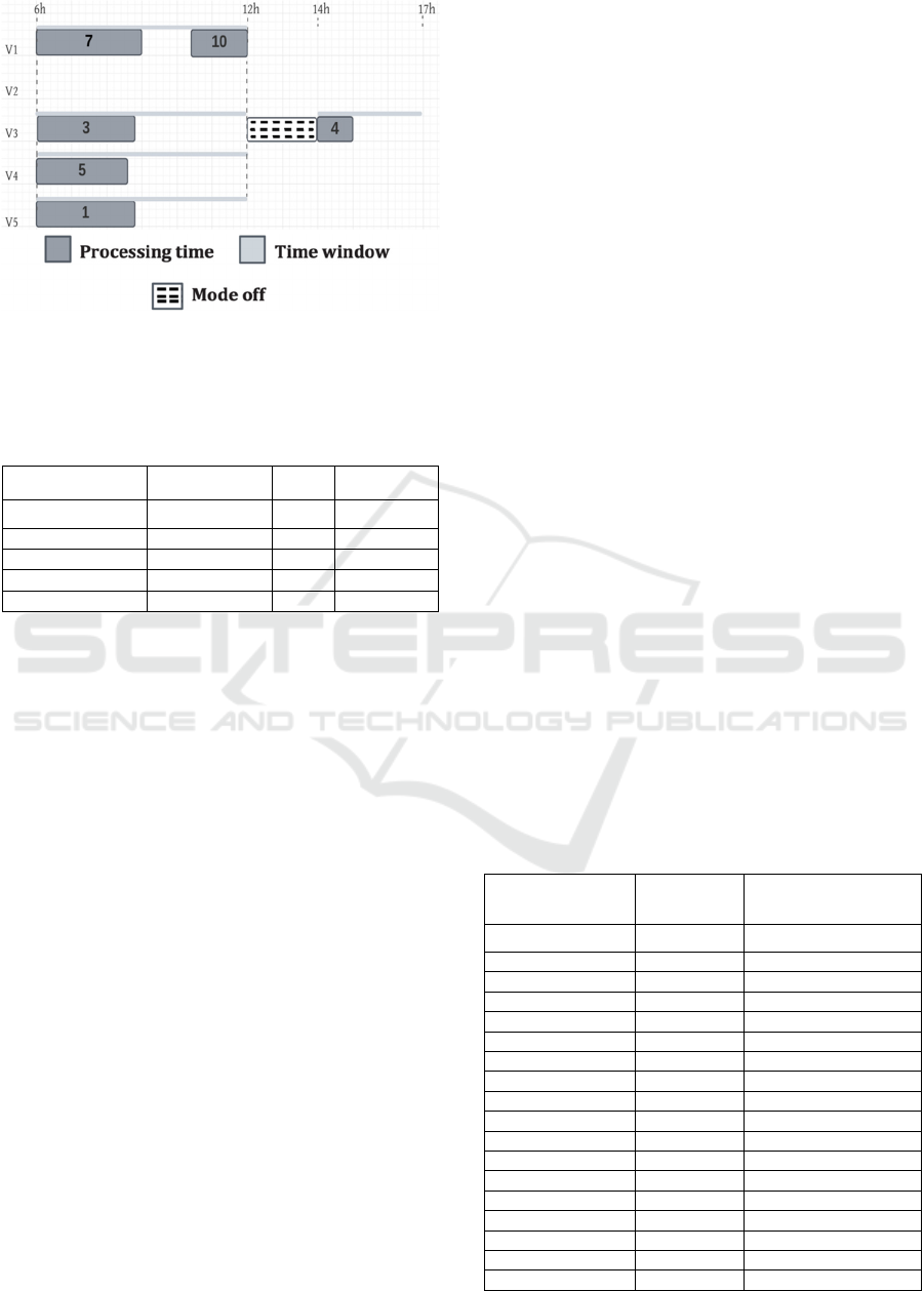
Figure 4: R10_1_F_P_1 - Gantt chart of the optimal
solution obtained by MIP2.
Table 7: R10_1_F_P_1-evaluation of MIP2 limit by
varying the number of tasks (NTF number of feasible
tasks).
Instances NS-n-NTF Obj Time (min)
R10_1_F_P_1 10-10-6 6 1.3
R10_1_F_P_2 10-15-10 10 30
R10_1_F_P_3 10-20-14 12 >120
R10_1_F_P_4 10-25-19 16 >120
R10_1_F_P_5 10-30-21 18 >120
Table 6 reveals that model 1 is more efficient in
computational time than model 2 on the illustrative
instance. We then investigated the limit of model 2 on
the same instance by duplicating the number of
requests of some sites to increase the number of tasks.
The results are summarized in table 7. The solutions
in bold are optimal, the others indicate the best
feasible solutions found by the solver while limiting
the computation time to 2h. We can see that model 2
can solve instances up to 15 tasks, 5 vehicles, 4 task
availability intervals and 3 vehicle availability
intervals. On instances with 20 tasks, the model
returns a feasible solution with about 85% of
completed tasks among all feasible tasks.
4.3 Comparison of MIP1 and MIP2
The purpose of this section is to study the limit of the
two models on 18 instances derived from a real case
study, and to compare their performance. Table 8
summarizes the obtained results. The columns MIP1-
obj and MIP2-obj give the percentage of tasks
performed in relation to the total number of tasks. It
can be noticed that both models have the same limit,
they succeed in solving optimally instances with up
to 15 tasks, 10 vehicles, 4 vehicle availability
intervals, and 3 task availability intervals. For
instances with 20 tasks, the table illustrates the best
feasible solutions found within a time limit of 2h.The
results show that model 2 performs better than model
1, the computation time on instances up to 15 tasks of
model 2 is on average 19% better compared to the
computation time of model 1. Model 1 takes from 3
to 90 minutes of computation time, while model 2
takes from 0.7 minutes to 37 minutes.
On the instances with 15 tasks, the computation
times are more important when using multiple
availability intervals compared to the instances with
only one vehicle availability interval. On instances
with 20 tasks, model 2 is able to satisfy up to 6% more
tasks compared to model 1. We can conclude that
model 2 is more efficient, and allowed us to solve up
to 15 tasks in a more reasonable time. We are
currently analyzing the obtained results, by
computing for each instance the real number of
feasible tasks, this will be used to adjust the objective
according to the feasible tasks, which is more
representative than using the total number of tasks.
These results have been validated by our industrial
partner. The obtained results are important for further
research which aims to solve larger instances. The
results of the MIP models will allow us to evaluate
heuristic approaches under development.
5 CONCLUSIONS
In this paper, we have presented a detailed study of a
new real problem encountered in the construction
sector on the optimization of waste bin transportation
in the framework of an organization with a
massification platform. The platform has a limited
Table 8a: Instances characteristics.
Instances NS-n-K [Min,Max]
DC, DV
R10_1_F_P_1 10-10-5 [1, 4] - [2, 3]
R10_2_F_P_1 10-10-5 [1, 4] - [2, 3]
R10_3_F_P_1 10-10-5 [1, 4] - [2, 3]
R10_1_F_U_1 10-10-5 [1, 4] - [1, 1]
R10_2_F_U_1 10-10-5 [1, 4] - [1, 1]
R10_3_F_U_1 10-10-5 [1, 4] - [1, 1]
R10_1_F_P_2 10-15-10 [1, 4] - [2, 3]
R10_2_F_P_2 10-15-10 [1, 4] - [2, 3]
R10_3_F_P_2 10-15-10 [1, 4] - [2, 3]
R10_1_F_U_2 10-15-10 [1, 4] - [1, 1]
R10_2_F_U_2 10-15-10 [1, 4] - [1, 1]
R10_3_F_U
_
2 10-15-10 [1, 4] - [1, 1]
R10_1_F_P_3 10-20-10 [1, 4] - [2, 3]
R10_2_F_P_3 10-20-10 [1, 4] - [2, 3]
R10_3_F_P_3 10-20-10 [1, 4] - [2, 3]
R10_1_F_U_3 10-20-10 [1, 4] - [1, 1]
R10_2_F_U_3 10-20-10 [1, 4] - [1, 1]
R10_3_F_U_3 10-20-10 [1, 4] - [1, 1]
Optimization of Direct Transportation Flows for the Removal of Construction Waste Bins with both Resource and Task Availability Interval
Constraints
227

Table 8b: Comparison of the performance of MIP1 and
MIP2.
Instances
NS-n-K MIP1
Obj.
MIP2
Obj.
MIP1
time
(min.)
MIP2
time
(min.)
R10_1_F_P_1 10-10-5 60% 60% 3 1.3
R10_2_F_P_1 10-10-5 50% 50% 5 1.5
R10_3_F_P_1 10-10-5 30% 30% 3 1.1
R10_1_F_U_1 10-10-5 10% 10% 4 1
R10_2_F_U_1 10-10-5 20% 20% 3.5 0.7
R10_3_F_U_1 10-10-5 20% 20% 3.7 0.9
R10_1_F_P_2 10-15_10 13% 13% 90 37
R10_2_F_P_2 10-15-10 33% 33% 66 30
R10_3_F_P_2 10-15-10 13% 13% 78 32
R10_1_F_U_2 10-15-10 7% 7% 57 28
R10_2_F_U_2 10-15-10 13% 13% 43 21
R10_3_F_U_2 10-15-10 7% 7% 53 26
R10_1_F_P_3 10-20-10 - 5%
>120 >120
R10_2_F_P_3 10-20-10 - 10%
>120 >120
R10_3_F_P_3 10-20-10 5% 5%
>120 >120
R10_1_F_U_3 10-20-10 5% 10%
>120 >120
R10_2_F_U_3 10-20-10 10% 15%
>120 >120
R10_3_F_U_3 10-20-10 5% 10%
>120 >120
fleet of heterogeneous vehicles available during
certain periods, the sites have a bin for each type of
waste and negotiate contracts with the platform for
the bin waste removal. The sites limit access to
vehicles at certain time windows periods. The
platform must manage the waste bin removal by
replacing each full bin with an empty bin. The
construction site may have multiple bin removal
requests (one request per bin waste type). We
modeled this problem as a scheduling problem on
non-identical parallel machines with new constraints
that concern the presence of multiple availability
intervals for both vehicles and tasks. We presented
two mathematical integer models, which we
compared and evaluated using 18 instances derived
from a real case study. The test results allowed us to
optimally solve instances up to 15 tasks, 10 vehicles,
4 task availability intervals and 3 vehicle availability
intervals. Currently, we are improving the
mathematical model by integrating the interval
incompatibility. The obtained results will allow us to
evaluate the quality of the heuristic approaches that
are under development.
REFERENCES
Jaballah, A., Ramdane Cherif-Khettaf, W. (2021). Multi-
trip Pickup and Delivery Problem, with Split Loads,
Profits and Multiple Time Windows to Model a Real
Case Problem in the Construction Industry. Proceeding
of ICORES 2021,pp. 200-207.
Ramdane Cherif-Khettaf, W., Jaballah,A, Ferri, F.(2022).
ILS-RVND Algorithm for Multi-trip Pickup and
Delivery Problem, with Split Loads, Profits and
Multiple Time Windows. ICCL 2022: 105-119 In: De
Armas, J., Ramalhinho, H., Voβ, S., (eds.), ICCL2022,
LNCS, vol 13557, pp.105-119, Springer.
Lenstra, J. K., Kan, A. R., & Brucker, P. (1977).
Complexity of machine scheduling problems. Annals of
Discrete Mathematics, 1, pp. 343–362.
Arık, O. A., Schutten, M., & Topan, E. (2022). Weighted
earliness/tardiness parallel machine scheduling
problem with a common due date. Expert Systems with
Applications, 187, 115916.
Osorio-Valenzuela, L., Pereira, J., Quezada, F., & Vásquez,
S. C. (2019). Minimizing the number of machines with
limited workload capacity for scheduling jobs with
interval constraints. Applied Mathematical Modelling,
74, pp. 512-527.
Suh-Jeng Yang (2013), Unrelated parallel-machine
scheduling with deterioration effects and deteriorating
multi-maintenance activities for minimizing the total
completion time, Applied Mathematical Modelling,
vol. 37-5, pp. 2995-3005.
Kaabi, Jihene, and Youssef Harrath (2014). A survey of
parallel machine scheduling under availability
constraints." International Journal of Computer and
Information Technology 3.2 pp. 238-245.
Gedik, R., Rainwater, C., Nachtmann, H., Pohl Ed A.,
(2016). Analysis of a parallel machine scheduling
problem with sequence dependent setup times and job
availability intervals. European Journal of Operational
Research 251.2, pp. 640-650.
ICORES 2023 - 12th International Conference on Operations Research and Enterprise Systems
228