Lightweight and Self Adaptive Model for Domain Invariant Bearing

Fault Diagnosis

Chandrakanth R Kancharla

1 a

, Jens Vankeirsbilck

1 b

, Dries Vanoost

2 c

, Jeroen Boydens

1 d

and Hans Hallez

1 e

M-Group, DistriNet, Department of Computer Science, KU Leuven Bruges Campus, 8200 Bruges, Belgium

M-Group, WaveCoRE, Department of Electrical Engineering, KU Leuven Bruges Campus, 8200 Bruges, Belgium

Keywords:

Condition Based Monitoring, Self Adaptation, Resource Constrained Computing, Bearing Fault Diagnosis,

Domain Invariance.

Abstract:

While the current machine fault diagnosis is affected by the rarity of cross conditional fault data in practice, ef-

ﬁcient implementation of these diagnosis models on resource constrained devices is another active challenge.

Given such constraints, an ideal fault diagnosis model should not be either generalizable across the shifting

domains or lightweight, but rather a combination of both, generalizable while being minimalistic. Prefer-

ably being uninformed about the domain shift. Addressing these computational and data centric challenges,

we propose a novel methodology, Convolutional Auto-encoder and Nearest Neighbors based self adaptation

(SCAE-NN), that adapts its fault diagnosis model to the changing conditions of a machine. We implemented

SCAE-NN for various cross-domain fault diagnosis tasks and compared its performance against the state-of-

the-art domain invariant models. Compared to the SOTA, SCAE-NN is at least 6−7% better at predicting fault

classes across conditions, while being more than 10 times smaller in size and latency. Moreover, SCAE-NN

does not need any labelled target domain data for the adaptation, making it suitable for practical data scarce

scenarios.

1 INTRODUCTION

Cloud computing is one of the major facilitators of

data analytics and intelligent decision making for in-

dustrial processes and machines. Although the com-

bination of IoT and cloud computing provides inﬁnite

computing and storage resources for the previously

remote machines, few challenges exist in fully cen-

tralizing the computation on the cloud (Wang et al.,

2020). Some critical challenges in the context of In-

dustrial IoT are, limited bandwidth, latency and reli-

ability of the connection. While IoT enabled devices

can continuously gather data from the machines and

their environments, their bandwidth availability lim-

itations cannot accommodate high data throughput.

This in combination with the latency of the data/ deci-

sion communication and connection reliability to the

https://orcid.org/0000-0002-1498-4296

https://orcid.org/0000-0003-0038-588X

https://orcid.org/0000-0002-7126-9758

https://orcid.org/0000-0002-7902-8537

https://orcid.org/0000-0003-2623-9055

cloud might lead to a catastrophe. Contrary to the

cloud, computing on the edge not only brings the la-

tency to ms scale but also reduces the overall opera-

tional costs by reducing the volume of data that has

to be migrated across the networks (Qiu et al., 2020).

With computing brought to the edge, the data is read-

ily available for knowledge extraction and faster deci-

sion making.

While edge computing can aid many time criti-

cal applications, bearing fault diagnosis is one ma-

jor ﬁeld that can readily beneﬁt from the low latency

computing at the edge. The components of a rotat-

ing machinery like a motor often fail, leading to com-

plete machine downtime or production quality reduc-

tion. According to Salah et al. (Salah et al., 2019),

up to 90% of small motors’ downtime is due to bear-

ing faults, and 40-44% for large motors. Real-time

characterization and detection of such frequently oc-

curring faults may allow the stake-holders to take an

appropriate and in-time action to avoid catastrophic

scenarios.

Summarizing the bearing fault diagnosis litera-

ture, the current State-Of-The-Art (SOTA) is majorly

Kancharla, C., Vankeirsbilck, J., Vanoost, D., Boydens, J. and Hallez, H.

Lightweight and Self Adaptive Model for Domain Invariant Bearing Fault Diagnosis.

DOI: 10.5220/0011822700003482

In Proceedings of the 8th International Conference on Internet of Things, Big Data and Security (IoTBDS 2023), pages 29-38

ISBN: 978-989-758-643-9; ISSN: 2184-4976

 2023 by SCITEPRESS – Science and Technology Publications, Lda. Under CC license (CC BY-NC-ND 4.0)

concentrated on deep learning models (Gawde et al.,

2022; Shan et al., 2022; Zhao et al., 2020). While

some of these proposed methods show impressive

performance, they ignore the fact that the data distri-

bution in practice may not always be the same as the

one used during the training (Pan and Yang, 2009).

The changing conditions of a machine, environmen-

tal noise, sensor deviation, etc can introduce domain

shift in the data. That is, the properties of the data do

not remain consistent across the training phase and

the real world inference. Thus leading to a deteri-

orated diagnostic model performance over the time.

Considering the above discussed restrictions, an ex-

emplary domain invariant model has to be efﬁcient

for the shifting domains while using as low computa-

tional resources as possible.

This article answers these aspects by:

• First, benchmarking the state-of-the-art domain

invariant methods for their performance, accu-

racy, latency and model footprint.

• Second, proposing a novel self adaptive fault di-

agnosis model and comparing it to the SOTA

models for both cross conditional efﬁciency and

computational resource usage.

The article is organised as follows. We brieﬂy

discuss the background of domain invariance in sec-

tion 2. Section 3 provides necessary details to un-

derstand the experimental setup. Section 4 discusses

the benchmark results. Which is followed by the pro-

posed methodology in Section 5. Section 6 and 7

summarizes the experimental results and conclusions

respectively.

2 BACKGROUND

There are predominantly three different research ar-

eas that investigate the domain invariance. They

are, learning domain invariant features from single-

source data, learning domain invariant features from

multiple-source data and lastly, domain adaptation

methods that re-adjust their prediction models to the

new domain.

If we consider that the data D

of an application is

available from three different domains k = 1,2, 3, the

data available for training in the form of source data

= D

{k}

is what will deﬁne these areas of diagnos-

tic model generalization research. Single-source do-

main generalization is where one domain’s data (D

1|2|3

) is used for model training and extracting do-

main invariant features that are generalizable across

the other two respective domains (D

= D

!1|!2|!3

Here | implies ’or’ and ! is ’not’. The effectiveness

of this strategy can be understood from works like

Yang et al., where they proposed a data augmentation

strategy to learn a generalizable deep neural network,

and our previous work, where we presented the usage

of latent features of a Convolutional Auto-encoder as

generalizable features across domains (Yang and Li,

2021; Kancharla et al., 2022).

Though the above discussed articles show the ef-

fectiveness of the single-source based generalization

models, Zheng et al. and An et al. suggest that the

multi-source domain based models are a practical ne-

cessity (Zheng et al., 2021; An et al., 2019). Multi-

source generalization involves considering multiple

source data (D

= D

1&2|2&3|3&1

) to train and test

generalizability performance on the left out domain

data (D

= D

3|1|2

). Here & represents ’and’. Var-

ious research results favor the argument of multi-

source domain generalization, but the fact that the

data is a scarce resource limits these methods in prac-

tice (Zheng et al., 2021; An et al., 2019; Zhang et al.,

2021; Zhao and Shen, 2022; Li et al., 2022).

To overcome the shortcomings of the single- and

multi-source generalization, domain adaption is pro-

posed. The domain adaptation method is where the

model trained with source domain data is adapted to

the other domains through model ﬁne tuning or distri-

bution alignment strategies in the feature space. Liu

et al. proposed an effective Domain Adversarial Neu-

ral Network (DANN) that can adapt to real world

data whilst being trained only with simulated bear-

ing fault data (Liu and Gryllias, 2022). Another study

by Li et al., studied the effectiveness of Central Mo-

ment Discrepancy (CMD) based domain adaptation

where the target domain data is assumed available but

without the class labels (Li et al., 2021). Maximum

Mean Discrepancy (MMD) and adversarial learning

based feature space adaptation (Wu et al., 2022) and

Multi Kernel-MMD based (Wan et al., 2022) strate-

gies are also effective and considered state-of-the-art.

Assessing the lack of uniformity and ease of compar-

ison, Zhao et al. studied various state-of-the-art do-

main adaptation methods in their comparative analy-

sis (Zhao et al., 2021).

Whilst being relatively high on data demand, do-

main adaptation can be considered more resilient and

safer option for achieving domain invariance as it

adapts rather than assumes. Which is not the case with

single and multi-source domain generalization mod-

els, they assume that domain invariant features exist

across new unknown conditions.

Even though the domain adaptation models are

relatively more employable in practice, it’s challeng-

ing to use them for two reasons. Firstly, the current

domain adaptation models for bearing fault diagnosis

IoTBDS 2023 - 8th International Conference on Internet of Things, Big Data and Security

use labelled target domain data to adapt. Which is in-

feasible to obtain in practice. The other reason is that

the adaptation process involve deep model relearning

which is computationally expensive. Whereas the real

world use cases necessitate implementation closer to

the edge, meaning low computational resource avail-

ability. These restrictions necessitate a new genre

of domain adaptation methodology that is accurate

across changing conditions whilst being computation-

ally efﬁcient. More importantly, it should not require

labelled target domain data for the adaptation.

Addressing the above mentioned restrictions, we

ﬁrst analysed the SOTA models for their cross condi-

tional efﬁciency and resource utilization. A new do-

main adaptation model is proposed based on Convo-

lutional Auto-encoder and Nearest Neighbours (CAE-

NN). The proposed model is computationally efﬁcient

compared to SOTA models. It has low latency predic-

tions, achieves better accuracy across conditions by

self adaptation and more importantly its simplistic do-

main adaptation routine has negligible computational

overhead compared to its inference.

3 EXPERIMENTAL SETUP

In this section we discuss the experimental setup used

for this investigation. First, various domain adapta-

tion methodologies from the literature that are worth-

while in terms of accuracy are introduced. Second,

various open source data-sets used for the perfor-

mance bench-marking are discussed. Finally, the de-

tails of the resources used for the experimentation are

provided.

3.1 Domain Invariant Models for

Comparison

Low data dependency during training is the major

consideration for choosing models for comparison in

this article. i.e., keeping the use-case as close to the

real-world as possible, we restricted this selection to

the models that use just the single-source data dur-

ing the training process. They are single-source do-

main generalization models and single-source domain

adaptation models.

3.1.1 Domain Generalization Models

From the literature, we consider two domain gener-

alization methods. While a Neural Network trained

on the data augmented samples proved to be domain

invariant in the case of (Yang and Li, 2021), the pro-

posal of Kancharla et al. was to use the latent features

of a CAE along with a K-Nearest Neighbors approach

as a domain invariant model (Kancharla et al., 2022).

Considering the provided results in the respective ar-

ticles, both approaches are considered for comparison

in this work.

3.1.2 Domain Adaptation Models

As discussed in Section 2, there are numerous pro-

posals and variations for domain adaptation, each for

a speciﬁc use-case or an application. Reproducing

and comparing them against each other was hard until

Zhao et al.’s work, where the authors compared com-

pared various domain adaptation strategies with a uni-

form data setting and model backbone. From their

benchmark study we understand that their are a few

competitive methodologies for different variations of

DA applications. Particularly for label consistent DA,

i.e., where labels in the source and target domain are

homogeneous, there are four methods that have con-

siderable performance. Multi kernel-Maximum Mean

Discrepancy (MK-MMD) is one of them, which re-

duces the marginal distributions of the source and

the target domains in the reproducing Hilbert Kernel

Space. Unlike MMD, MK-MMD uses multiple ker-

nels to embed the feature space and minimize the dis-

tance between the marginal distributions of the source

and the target domain (Gretton et al., 2012). The

other feature alignment method is based on adapt-

ing the model to the target domain by reducing both

the marginal and conditional distributions between

the source and target domains, it is referred to as

Joint MMD (JMMD) (Long et al., 2016). While the

models mentioned above were competitively placed

in terms of performance, the domain adversarial loss

minimization based methods like Domain Adversar-

ial Neural Network (DANN) and Conditional Domain

Adversarial Network (CDAN) demonstrated overall

best mean performance (Zhao et al., 2021). They re-

spectively introduce and minimize marginal and joint

adversarial loss of the Neural Network model train-

ing through a domain discriminator. The reduced loss

thus results in a model that is domain agnostic.

An important aspect of these domain alignment

or adversarial models is having an appropriate feature

extractor, also referred to as the backbone model. A

good backbone leads to a better feature representa-

tions and eventually better domain adaption possibil-

ities.

3.1.3 Backbone Model

Although numerous deep neural network architec-

tures exist, we restricted this study to just two deep

models to compare the above selected methods. Thus,

Lightweight and Self Adaptive Model for Domain Invariant Bearing Fault Diagnosis

four best performing adaptation methods in combina-

tion with two different deep feature extractors will be

used to benchmark and compare. We included the re-

sults of both standard Convolutional Neural Network

(CNN) and RESNET 18 backbones in this study to

quantify and appropriately discuss the trade-off be-

tween the model size and the efﬁciency of domain

adaptation. The same CNN architecture is used for

the shadow label based domain generalization evalua-

tion to remove any architectural advantage. Whereas,

the model architecture of the CAE from CAE-NN is

consistent to the original paper as it is an unsuper-

vised feature learner and is different to the other meth-

ods considered here (Kancharla et al., 2022). The

summary of the architectures used and their respec-

tive Floating Point Operations (FLOPs) necessary for

inferring one input of size (1,256) is presented in Ta-

ble 1. We can see from Table 1 that CAE network

used for inference is much shallower compared to the

CNN and RESNET, making the concept of architec-

tural advantage irrelevant.

Table 1: Backbone models’ architecture and FLOPs for a

256 input size.

Model Architecture MFLOPs

RESNET 18

⊛

‡

⋆

46.19

CNN 4

⊛

‡

⋆

4.37

CAE 2

⊛

‡

⋆

0.32

⊛

convolution layers;

‡

pooling layers;

⋆

f ully connected/dense layers;

batch normalization layers

3.2 Datasets

Various open-source bearing fault datasets are ideal

for algorithmic evaluation (Zhao et al., 2020). In

this paper, we will use two datasets with extensive

vibration data, the Case Western Reserve University

dataset (CWRU) and the Paderborn University dataset

(PU) (Lessmeier et al., 2016; Smith and Randall,

2015). While the (CWRU) dataset is frequently used

in the studied literature, (PU) is also widely referred.

With four different conditions (load = 0,1,2,3 Hp)

and 10 different faulty and non-faulty classes, the

CWRU dataset can be considered relatively easy to

diagnose (Zhao et al., 2020). While the provided data

ﬁles consist of vibration data sampled at 12 kHz and

48 kHz from both the motor’s driving and fan end,

only the drive end data collected at 12 kHz is used in

this study.

Whereas, the PU dataset has a unique combina-

tion of machine conditions that vary in multiple di-

mensions. Rotating speed (1500 and 900 RPM), ap-

plied Radial force (1000 and 400 N) and Load torque

(0.7 and 0.1 Nm). With four different combinations

of the three variables as mentioned above, PU dataset

entails 6 healthy classes, 12 artiﬁcial fault classes and

14 natural run to failure fault classes. Each of these

class’ data is collected for four seconds at 64 kHz

for 20 times. Given the large amount of data for the

PU dataset, randomly selected ﬁve ﬁles of each class

were used for training and testing. Notably, the aver-

age accuracies across some of the state-of-the-art do-

main adaptation methodologies on PU dataset is very

low (Zhao et al., 2021). This makes it one of the most

complex datasets currently available to validate do-

main invariance.

3.2.1 Experimental Tasks

Given four different conditions in CWRU and PU

datasets each, there are 12 different experimental

tasks possible individually. Each experimental task

is deﬁned as, one condition’s data within a dataset

as training data and another condition’s data within

the same dataset as test data. While all the 24 tasks

have been experimented with, we summarize the re-

sults with one critical task from each dataset to re-

duce the overwhelming amount of information. The

critical task here is deﬁned by the transfer of informa-

tion across majorly different conditions. According

to our experiments and the benchmark study (Zhao

et al., 2021) these critical tasks are C3-C0 and P2-

P0 from CWRU and PU datasets respectively. C3-C0

refers to CWRU load condition 3 Hp as source/ train

data and load condition 0 Hp as target/ test data, simi-

larly, P2-P0 is PU dataset condition 2 (1500 RPM, 0.1

Nm and 1000 N) as source/ train data to condition 0

(900 RPM, 0.7 Nm and 1000 N) as target/ test data.

Thus in this study the results of these two tasks will

be discussed.

3.2.2 Model Inputs and Pre-Processing

Frequency-based features have been proven to be

good in modelling the data for domain adaptation and

generalization characteristics (Zhao et al., 2021; Kan-

charla et al., 2022). Following that understanding,

we used frequency transformed data as the model in-

puts. As the considered data is continuous in nature

and assuming each sample window contains at least

one spindle rotation’s information, the selected sam-

ple windows for CWRU and PU data ﬁles are chosen

to be 512 and 2048 sample points respectively. Fast

Fourier Transform has been applied on these windows

and absolute values of the positive spectrum are re-

tained. Finally, they are introduced to the appropriate

models as inputs (256 and 1024 for CWRU and PU re-

spectively). Whereas its outputs are 10 class labels of

IoTBDS 2023 - 8th International Conference on Internet of Things, Big Data and Security

CWRU (1 normal and 9 faulty) and 14 class labels of

PU (1 normal and 13 faulty), are also provided to the

model during training and target labels as inputs while

domain adaptation with CNN and RESNET backed

methods. Training and testing data from both source

domain and target domain are split into 80-20. All

the training and retraining happen with the 80 split

data while the testing is done on the 20 split.

3.2.3 Performance Evaluation Metrics

Model efﬁcacy was measured and evaluated based on

the general accuracy, i.e. the amount of correctly pre-

dicted samples out of all samples across conditions.

Whereas, the model computational efﬁciency was

mostly measured by various parameters like model

size, number of operations performed, and inference

latency. Model size was measured in terms of the

memory consumed by the trainable and non-trainable

parameters involved in model inference. Number

of Floating Point Operations (FLOPs) per inference

were also gathered to understand the computational

complexity of the models. Additionally, per sample

inference latency was measured, i.e, time taken for

inferring each randomly selected sample. Except for

data pre-processing, this latency measure includes all

the steps for per sample feature extraction and classi-

ﬁcation. Moreover, for each model evaluated in this

study, these metrics were collected from 3 separate

experiments to eliminate any bias due to randomness.

3.3 Experimental platform

Both model characterization of the selected SOTA

methods and preliminary analysis of the proposed

self adaptive method have been performed on a com-

puter with Intel® i7-8850H CPU running at 2.60GHz,

equipped with 32GB RAM. Please note, as the ex-

perimental platform does not represent a constrained

device, we infer and discuss the computational efﬁ-

ciency of the SOTA models based on the acquired

computing parameters from the experiments. None

of the acquired computational parameters vary across

devices, except for the latency.

4 RESULTS OF MODEL

BENCHMARKING

We ﬁrst performed an end to end benchmark study

for the various SOTA models upon the experimental

tasks discussed above. As mentioned previously, the

end to end performance study involved analyzing pa-

rameters like model footprint, FLOPs, accuracy and

per sample inference latency. From Table 2, we can

observe that the RESNET backed domain adaptation

models are in general 15-30% more accurate than the

CNN features based models. But there is a large dif-

ference in the FLOPs, model size and the latency of

inference between them. While the aggregate num-

ber of operations performed by CNN based models

are approximately 4.37 M and 18.1 M for both the

cases respectively, for the same tasks the RESNET

model needs to perform approximately 10 times more

FLOPs. On the other hand, latency of RESNET mod-

els is .approximately 4 times to that of CNN mod-

els within the dataset. Inference latency and FLOPs

of similar models are different across the datasets be-

cause of the change in the number of inputs. As dis-

cussed in the previous section, CWRU has 256 inputs

while PU has 1024 inputs, which are 4 times more

compared to CWRU, leading to more computations

performed. Whereas, the trainable parameters and

model size does not change across the tasks as they

are architectural parameters and are independent of

the input size.

As opposed to RESNET and CNN based mod-

els, the single domain generalization model, CAE-NN

is competitively placed in terms of accuracy whilst

having smaller space requirements, lower number

of performed operations and inference latency. It’s

the second best performing model with CWRU task

and better than the CNN models for the PU task.

When compared to CAE-NN, RESNET backed mod-

els are slightly effective at cross domain adaptation,

but CAE-NN is several orders less complex. It is

100 times lower on number of FLOPs and approxi-

mately 10 times low on prediction latency compared

to RESNET models. Overall, even though it is a

single-source domain generalization model, it’s evi-

dent that CAE-NN has the best accuracy over infer-

ence latency and FLOPs ratios out of all the domain

invariant SOTA models.

Summarizing the SOTA domain invariant mod-

els for resource constrained implementation, we

found that the data augmentation based method

showed the least cross-domain generalization capa-

bility. Whereas the labelled target data based domain

adaption of CNN models’ performance is mediocre.

Finally, RESNET backed models are the best per-

forming for the considered tasks and show very high

adaptability to the changing conditions. But this is

at the cost of labelled target data, which is scarce in

practice as discussed in the previous section. The next

best model CAE-NN does this generalization without

any prior knowledge of the feature distribution in the

target domain. Additionally, the number of trainable

parameters that have to be accommodated on a com-

Lightweight and Self Adaptive Model for Domain Invariant Bearing Fault Diagnosis

Table 2: Cross conditional bearing fault diagnosis models’ performance and their corresponding computational metrics.

Model Accuracy (%) Latency (ms) FLOPs (Million) Model size (MB) Params (Thousand)

Task: CWRU C3-C0; input size: 256

CAE-NN 92.2 0.2 0.42 0.20 26.61

C-Shadow 69.5 0.5 4.37 0.93 232.90

C-CDAN 82.6 0.6 4.37 0.93 232.90

C-DAN 79.7 0.7 4.37 0.93 232.90

C-MKMMD 74.3 0.6 4.37 0.93 232.90

C-JMMD 79.1 0.6 4.37 0.93 232.90

R-CDAN 93.5 3.0 46.19 15.91 3977.80

R-DAN 89.9 3.0 46.19 15.91 3977.80

R-MKMMD 84.7 3.0 46.19 15.91 3977.80

R-JMMD 83.1 3.0 46.19 15.91 3977.80

Task: PU P2-P0; input size: 1024

CAE-NN 41.8 0.3 1.66 0.80 98.61

C-Shadow 34.6 1.2 18.10 0.93 233.93

C-CDAN 39.2 1.1 18.10 0.93 233.93

C-DAN 39.3 1.0 18.10 0.93 233.93

C-MKMMD 43.2 1.2 18.10 0.93 233.93

C-JMMD 41.0 1.3 18.10 0.93 233.93

R-CDAN 53.6 4.3 184.39 15.91 3978.83

R-DAN 48.1 4.0 184.39 15.91 3978.83

R-MKMMD 58.7 4.0 184.39 15.91 3978.83

R-JMMD 78.2 4.0 184.39 15.91 3978.83

C − /R − Pre f ix denotes backbones used, C : CNN; R : RESNET 18.

putational platform is an unfair comparison between

the RESNET backed models and CAE-NN. Trainable

prameters of RESNET are approximately 20 times

more compared to CNN and more than 40 times com-

pared to CAE-NN.

5 PROPOSED

SELF-ADAPTATION

STRATEGY

Taking advantage of the generalization prowess of

CAE-NN we devised a self adaptive strategy as vrep-

resented in Figure 1. From the benchmark experi-

ments conducted on CAE-NN, there is enough evi-

dence to consider that the source domain (D

) and the

target domain (D

) share similar feature distribution

or at least have a close proximity in the latent space

L. This is valid for the two tasks considered here that

are very different in their conditions and for the ma-

jority of the 24 cases from both CWRU and PU tasks.

We can observe that a considerate amount of samples

are accurately classiﬁed across the domains. Thus,

we propose to use this new found information from

across the domain to retrain the existing CAE-NN.

And the so re-trained CAE-NN will be called SCAE-

NN (Self adapted CAE-NN).

But, taking into account the low computational re-

source availability at the edge, our proposal will con-

sider re-training the classiﬁer alone, KNN in this case.

The proposal involves three simple steps,

• Inferring a new sample.

• Pseudo label the strong predictions.

• Retrain the KNN with pseudo labelled predic-

tions.

In other words, if a sample X

, an i

sample of the

target domain D

is predicted with probability above

a threshold, it will be considered a strong prediction.

The latent features of this strong prediction i.e, l

ac-

quired from the encoder will be pseudo labelled as Y

As a retraining step, this pseudo labelled set of (data,

label {l

}) pair will be added to the KNN training

set KNN

As we are using the KNN with brute force ap-

proach, the retraining phase of the KNN in the pro-

posed SCAE-NN is simply appending the new (data,

label) pair to the existing pairs. This means, the

proposed re-training method of SCAE-NN can be

implemented with a negligible amount of computa-

tional overhead compared to the inference of CAE-

NN. While the KNN re-training can be performed

with the similar cost of inference, its trade-off will

be elaborated in the next section.

IoTBDS 2023 - 8th International Conference on Internet of Things, Big Data and Security

Raw data

Condition X

FFT Scaler

Pre-processing

Feature extraction & classification

Back propogation

Encoder Latent features Decoder

KNN Classifier

Raw data

Condition Y

FFT Scaler

Encoder Latent features

KNN Classifier

Training

Testing

Class probability >0.9

Pseudo label

(data, label) pair

Self-adaptation

Figure 1: Block diagram describing the proposed self-adaptation strategy utilizing the generalizability of CAE-NN and pseudo

labelling.

Probability Threshold

In general, the ﬁnal prediction of KNN is based on

the maximum number of K closest neighbours in the

feature space. Whereas for the re-learning purpose

we pseudo label only the strong predictions. Strong

predictions here mean the samples that are predicted

with over certain probability threshold. Although the

threshold selection is dynamic and subjective to do-

main adaptation use case, in this article we chose

probability over 0.9 for pseudo labelling a sample.

This in some cases might not produce high rate of

adaptation, but restricts negative learning by consid-

ering only the strong positive predictions.

6 RESULTS

As mentioned in the experimental setup section, all

the performance evaluation metrics for the proposed

SCAE-NN were also acquired from 3 individual ex-

periments for each task and mean values are reported.

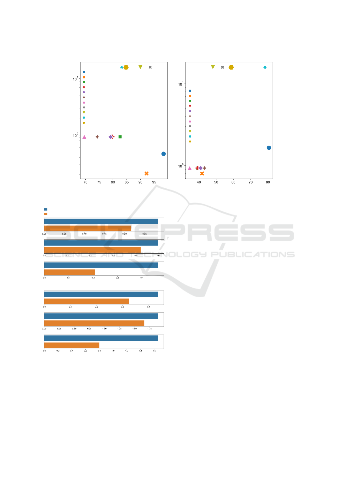
Figure 2 compares the SOTA domain invariant mod-

els discussed in the previous section to the self-

adaptive model proposed in this article SCAE-NN.

Starting with the improvement over CAE-NN, self-

adaptive version is approximately 8-9% more accu-

rate for C3-C0 task and an impressive 35-40% higher

for the P2-P0 task. Empirical results suggest that the

proposed SCAE-NN is capable of adapting to the new

conditions much better than the SOTA domain adap-

tation models. It adapts 6-7% better than best per-

forming RESNET backed models for C3-C0 task and

2-3% for P2-P0. This is a signiﬁcant improvement

over the SOTA models in terms of accuracy.

Moreover, the model sizes of SCAE-NN com-

pared to the RESNET based models are substantially

low. It is approximately 33.4 and 9.3 times smaller for

(1,256) and (1,1024) respective inputs of the CWRU

and PU tasks. While the model size does not change

with the inputs in the case of RESNET or CNN mod-

els, SCAE-NN’s does vary. As can be seen from

Figure 3, the effect of SCAE-NN retraining is rela-

tively high on the model size, latency of prediction

and ﬂoating point operations. This is more drastic in

the case of model size compared to the latency and

FLOPs.

Both the input size and the number of samples

used during training and re-training affect the model

size of SCAE-NN because of the KNN. While KNN

does not ﬁt any function to the data during training,

it searches its feature space during every inference.

KNN evaluates the new data point’s distance from ev-

ery other data point in the training set during infer-

ence. Thus, after the retraining of SCAE-NN, newly

added pseudo samples lead to increased model size

and introduce extra computations during inference.

The increased computational overhead during in-

ference is reﬂected by the increased Latency and

FLOPs of SCAE-NN. While the average FLOPs

count was 0.41 and 1.62 Million with CAE-NN for

CWRU and PU tasks respectively, with SCAE-NN it

has increased by up to 0.1-0.2 Million for both the

tasks. Also a similar increase on the latency of per

sample inference can be observed. Figure 4 shows pe-

riodic increase in the accuracy and the inference time

Lightweight and Self Adaptive Model for Domain Invariant Bearing Fault Diagnosis

Accuracy (%) Accuracy (%)

Model size (MB)

C3-C0 P2-P0

R-CDAN

C-DAN

CAE-NN

C-CDAN

C-JMMD

C-MKMMD

C-Shadow

R-DAN

R-JMMD

R-MKMMD

DA model

SCAE-NN

R-CDAN

C-DAN

CAE-NN

C-CDAN

C-JMMD

C-MKMMD

C-Shadow

R-DAN

R-JMMD

R-MKMMD

DA model

SCAE-NN

Model size (MB)

Figure 2: Comparison of the domain invariant models for their model sizes against the accuracies. With considerably low

model size, SCAE-NN is at par or sometimes better than RESNET based domain adaptation models.

Time (ms)

FLOPs (M)

Model size (MB)

Time (ms)

FLOPs (M)

Model size (MB)

CAE-NN

SCAE-NN

b) PU

a) CWRU

Figure 3: Across CAE-NN and SCAE-NN, we can observe

an exponential increase in the model size compared to the

linear increase in the latency and number of operations.

with changing number of new observations used in

retraining.

From Figure 4, we can see that about 80-90% of

the adaptation is due to the ﬁrst 40-50% of the new

observations. Particularly, for the PU task this adap-

tation is around 90% by the 40% mark. The accuracy

gain after that point is a trade-off with the increased

model size and latency. Nevertheless, summarizing

the results from Figures 2 and 3, with better accura-

cies, lower number of FLOPs, low latency of infer-

ence and lower model size than the RESNET models,

SCAE-NN is the best choice for any application that

is resource constrained or not.

The adapted fault diagnosis model of CWRU task

is very close to being perfect. Whereas, the PU task

still has some room for fault diagnosis adaptation.

Figure 5 represents the confusion matrix of PU task

after SCAE-NN adaptation, It is clear that all the nor-

mal classes i.e, label number ’13’ from the ﬁgure are

predicted correctly. Most of the other faulty classes

are also appropriately classiﬁed. Even though the

miss classiﬁcations amongst the faulty classes doesn’t

affect the overall fault predictability. The frequently

occurring and note worthy confusion is between class

number 4, KA30, generated by ’plastic deformation:

indentation’ and the normal class. It has to be un-

derstood well to further improve the cross conditional

bearing fault diagnosis performance. The next impor-

tant case that needs further understanding is between

class numbered 6, originally KA24 generate by fa-

tigue pitting and the normal class. While the KA30 is

non severe fault case, the KA24 is a severe one with

faults on both inner race and outer race. While the

general expectations are that these strong fault cases

are classiﬁed apart from normal classes, it is unclear

of why these two classes are confused with the nor-

IoTBDS 2023 - 8th International Conference on Internet of Things, Big Data and Security

Observation number

Latency (ms)

Accuracy (%)

a) CWRU

b) PU

Latency (ms)

Accuracy (%)

Observation number

Figure 4: Periodic increase in the accuracy with the new

observation based KNN retraining. We also observe the in-

creasing per sample inference latency due to the increased

KNN samples.

Figure 5: Confusion matrix of PU task after the self adapta-

tion with SCAE-NN.

mal ones. Might be a case of negative learning, and

need to be further investigated.

For the readers interested in the class labels as

mentioned in the original PU dataset paper (Smith

and Randall, 2015), the chronological order of 0-12

classes mentioned in Figure 5 are ’KA04’, ’KA15’,’

KA16’, ’KA22’, ’KA30’, ’KB23’, ’KB24’, ’KB27’,

’KI14’, ’KI16’, ’KI17’, ’KI18’, ’KI21’ and all the six

non faulty classes are label 13.

7 CONCLUSIONS AND FUTURE

WORK

In this article, we ﬁrst analysed various SOTA mod-

els of bearing fault diagnosis for domain invariance.

This was particularly performed from the perspective

of resource deﬁcient implementation. Different met-

rics concerned with cross conditional fault classiﬁca-

tion performance and implementability were used to

benchmark them. First, from the benchmark study it

is evident that the current models are limited either

based on their performance or computational com-

plexity. Overall, domain adversarial methods and dis-

tribution alignment methods based on RESNET fea-

tures were the best performing. Whereas the same

strategies with features from less complex CNN ar-

chitecture were competitively placed after RESNET

models. Relative to CNN and RESNET based mod-

els, CAE-NN, an Auto-encoder and K-Nearest Neigh-

bors based domain generalization model was compu-

tationally efﬁcient while exhibiting promising cross

fault diagnosis accuracies.

Additionally, a new self adaptation methodology

SCAE-NN based on CAE-NN has been proposed.

Its performance evaluation for cross conditional do-

main adaptation was conducted and the results were

reported. The proposed novel methodology demon-

strated impressive self adaptive nature. While other

performance metrics like inference latency, model

size and FLOPs were relatively high compared to the

non adapted model CAE-NN, the accuracy improve-

ments were at least 8%-40% higher for the evaluated

tasks. What is more impressive is that the SCAE-

NN is self-supervised, whereas the compared models

are supervised. Despite the fact that it is unfair, the

authors chose to compare it to supervised adaptation

models because they are the SOTA for domain invari-

ant fault diagnosis.

Although SCAE-NN is several orders less com-

plex than the next best method, there is a scope to

further improve it in terms of resource utilization efﬁ-

ciency and will the subject of our future work. Ad-

ditionally, future implementation and characteriza-

tion of SCAE-NN will be performed using micro-

controllers, which are the epitome of resource con-

strained edge.

ACKNOWLEDGEMENT

This work is supported by the VLAIO-PROEFTUIN

”Industry 4.0 Machine Upgrading” (Project num-

ber:180493).

Lightweight and Self Adaptive Model for Domain Invariant Bearing Fault Diagnosis

REFERENCES

An, Z., Li, S., Wang, J., Xin, Y., and Xu, K. (2019). Gener-

alization of deep neural network for bearing fault di-

agnosis under different working conditions using mul-

tiple kernel method. Neurocomputing, 352:42–53.

Gawde, S., Patil, S., Kumar, S., Kamat, P., Kotecha, K., and

Abraham, A. (2022). Multi-fault diagnosis of indus-

trial rotating machines using data-driven approach: A

review of two decades of research.

Gretton, A., Sriperumbudur, B. K., Sejdinovic, D., Strath-

mann, H., Balakrishnan, S., Pontil, M., and Fukumizu,

K. (2012). Optimal kernel choice for large-scale two-

sample tests. In NIPS.

Kancharla, C. R., Vankeirsbilck, J., Vanoost, D., Boydens,

J., and Hallez, H. (2022). Latent dimensions of auto-

encoder as robust features for inter-conditional bear-

ing fault diagnosis. Applied Sciences, 12(3):965.

Lessmeier, C., Kimotho, J., Zimmer, D., and Sextro, W.

(2016). Condition monitoring of bearing damage in

electromechanical drive systems by using motor cur-

rent signals of electric motors: A benchmark data set

for data-driven classiﬁcation.

Li, J., Shen, C., Kong, L., Wang, D., Xia, M., and Zhu,

Z. (2022). A new adversarial domain generalization

network based on class boundary feature detection for

bearing fault diagnosis. IEEE Transactions on Instru-

mentation and Measurement, 71:1–9.

Li, X., Hu, Y., Zheng, J., Li, M., and Ma, W. (2021). Cen-

tral moment discrepancy based domain adaptation for

intelligent bearing fault diagnosis. Neurocomputing,

429:12–24.

Liu, C. and Gryllias, K. (2022). Simulation-driven do-

main adaptation for rolling element bearing fault di-

agnosis. IEEE Transactions on Industrial Informatics,

18(9):5760–5770.

Long, M., Zhu, H., Wang, J., and Jordan, M. I. (2016). Deep

transfer learning with joint adaptation networks.

Pan, S. J. and Yang, Q. (2009). A survey on transfer learn-

ing. IEEE Transactions on knowledge and data engi-

neering, 22(10):1345–1359.

Qiu, T., Chi, J., Zhou, X., Ning, Z., Atiquzzaman, M.,

and Wu, D. O. (2020). Edge computing in industrial

internet of things: Architecture, advances and chal-

lenges. IEEE Communications Surveys & Tutorials,

22(4):2462–2488.

Salah, A. A., Dorrell, D. G., and Guo, Y. (2019). A re-

view of the monitoring and damping unbalanced mag-

netic pull in induction machines due to rotor eccen-

tricity. IEEE Transactions on Industry Applications,

55(3):2569–2580.

Shan, N., Xu, X., Bao, X., and Qiu, S. (2022). Fast fault

diagnosis in industrial embedded systems based on

compressed sensing and deep kernel extreme learning

machines. Sensors, 22(11):3997.

Smith, W. A. and Randall, R. B. (2015). Rolling ele-

ment bearing diagnostics using the case western re-

serve university data: A benchmark study. Mechani-

cal Systems and Signal Processing, 64-65:100–131.

Wan, L., Li, Y., Chen, K., Gong, K., and Li, C. (2022).

A novel deep convolution multi-adversarial domain

adaptation model for rolling bearing fault diagnosis.

Measurement, 191:110752.

Wang, X., Han, Y., Leung, V. C. M., Niyato, D., Yan, X.,

and Chen, X. (2020). Convergence of edge computing

and deep learning: A comprehensive survey. IEEE

Communications Surveys & Tutorials, 22(2):869–904.

Wu, Y., Zhao, R., Ma, H., He, Q., Du, S., and Wu, J. (2022).

Adversarial domain adaptation convolutional neural

network for intelligent recognition of bearing faults.

Measurement, 195:111150.

Yang, Y. and Li, C. (2021). Quantitative analysis of

the generalization ability of deep feedforward neural

networks. Journal of Intelligent & Fuzzy Systems,

40(3):4867–4876.

Zhang, Q., Zhao, Z., Zhang, X., Liu, Y., Sun, C., Li, M.,

Wang, S., and Chen, X. (2021). Conditional adversar-

ial domain generalization with a single discriminator

for bearing fault diagnosis. IEEE Transactions on In-

strumentation and Measurement, 70:1–15.

Zhao, C. and Shen, W. (2022). A domain generalization

network combing invariance and speciﬁcity towards

real-time intelligent fault diagnosis. Mechanical Sys-

tems and Signal Processing, 173:108990.

Zhao, Z., Li, T., Wu, J., Sun, C., Wang, S., Yan, R., and

Chen, X. (2020). Deep learning algorithms for rotat-

ing machinery intelligent diagnosis: An open source

benchmark study. ISA Transactions.

Zhao, Z., Zhang, Q., Yu, X., Sun, C., Wang, S., Yan, R.,

and Chen, X. (2021). Applications of unsupervised

deep transfer learning to intelligent fault diagnosis: A

survey and comparative study. IEEE Transactions on

Instrumentation and Measurement, 70:1–28.

Zheng, H., Yang, Y., Yin, J., Li, Y., Wang, R., and Xu,

M. (2021). Deep domain generalization combining a

priori diagnosis knowledge toward cross-domain fault

diagnosis of rolling bearing. IEEE Transactions on

Instrumentation and Measurement, 70:1–11.

IoTBDS 2023 - 8th International Conference on Internet of Things, Big Data and Security