A Concept for Optimal Warehouse Allocation Using Contextual

Multi-Arm Bandits

Giulia Siciliano

, David Braun

, Korbinian Zöls

and Johannes Fottner

Chair of Materials Handling, Material Flow, Logistics, Technical University of Munich, Garching bei München, Germany

Institute of Flight System Dynamics, Technical University of Munich, Garching bei München, Germany

Keywords: Artificial Intelligence, Machine Learning, Warehouse Management, Storage Strategies.

Abstract: This paper presents and demonstrates a conceptual approach for applying the Linear Upper Confidence Bound

algorithm, a contextual Multi-arm Bandit agent, for optimal warehouse storage allocation. To minimize the

cost of picking customer orders, an agent is trained to identify optimal storage locations for incoming products

based on information about remaining storage capacity, product type and packaging, turnover frequency, and

product synergy. To facilitate the decision-making of the agent for large-scale warehouses, the action selection

is performed for a low-dimensional, spatially-clustered representation of the warehouse. The capability of the

agent to suggest storage locations for incoming products is demonstrated for an exemplary warehouse with

4,650 storage locations and 30 product types. In the case study considered, the performance of the agent

matches that of a conventional ABC-analysis-based allocation strategy, while outperforming it in regards to

exploiting inter-categorical product synergies.

1 INTRODUCTION

Considering that warehousing constitutes the most

cost-intensive part of modern supply chains (Rushton

et al., 2010), efficient warehouse operation is of

paramount importance to supply chain management.

A large portion of the total warehouse operating costs

usually results from the picking of goods. For

example, in (de Koster et al., 2007) it is estimated that

picking of goods accounts for 55% of the total

warehouse operating costs. To minimize this cost,

various picking strategies were developed. A

discussion of common routing methods is provided in

(Petersen and Aase, 2004). Because the picking costs

of a product are largely determined by its position in

the warehouse, a large portion of the picking costs can

be traced back to the storage allocation of the product

after its arrival in the warehouse. In (Heragu et al.,

2005) a mathematical model and heuristics were

developed to determine the optimal allocation of

products in the different functional areas of a

warehouse, considering also their respective size. To

https://orcid.org/0000-0002-8438-9409

https://orcid.org/0000-0003-1873-2069

https://orcid.org/0000-0002-2998-9890

https://orcid.org/0000-0001-6392-0371

solve the problem of optimal allocation in

warehouses, in (Jiao et al., 2018) a multi-population

genetic algorithm is successfully developed and

applied.

To minimize the cost of warehouse operation, we

suggest the application of the Linear Upper

Confidence Bound (LinUCB) algorithm (Li et al.,

2010), a contextual Multi-arm Bandit method, for

optimizing the storage allocation of incoming goods

in large-scale warehouses. Specifically, an Artificial

Intelligence (AI) agent is trained to identify feasible

storage locations for incoming products that, with

regard to the current state of the warehouse and the

characteristics of the item to be stored, minimize the

expected time required to pick future customer

orders.

The remainder of the paper is structured as

follows. Firstly, in Section 2, the proposed AI-based

storage allocation strategy is presented in detail. Its

performance in an exemplary warehouse with 4,650

storage locations and 30 product types is

demonstrated throughout Section 3. Final conclusions

460

Siciliano, G., Braun, D., Zöls, K. and Fottner, J.

A Concept for Optimal Warehouse Allocation Using Contextual Multi-Arm Bandits.

DOI: 10.5220/0011839700003467

In Proceedings of the 25th International Conference on Enterprise Information Systems (ICEIS 2023) - Volume 1, pages 460-467

ISBN: 978-989-758-648-4; ISSN: 2184-4992

 2023 by SCITEPRESS – Science and Technology Publications, Lda. Under CC license (CC BY-NC-ND 4.0)

and suggestions for future research are provided in

Section 4.

2 METHOD

The proposed method addresses the problem of

optimal storage allocation in two stages. In the first

stage, the LinUCB algorithm is applied. Here, to

facilitate the operations of the agent in large-scale

warehouses, the decision-making is performed for a

low-dimensional representation of the warehouse,

obtained by BIRCH clustering (Zhang et al., 1996).

Thus, instead of allocating incoming products to

specific storage locations, the LinUCB agent assigns

incoming products to spatial warehouse clusters.

Subsequently, in the second stage of the decision-

making, a heuristic decision rule is applied to allocate

the incoming product to a specific storage location

within the previously selected spatial cluster.

2.1 Pre-processing: Spatial Clustering

of Warehouse Locations

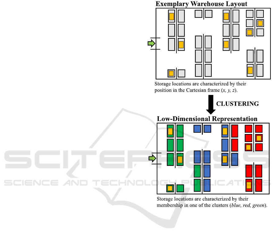
The spatial clustering of the warehouse locations into

spatially similar clusters acts as the pre-processing

stage of the presented AI-based optimal storage

allocation method and, as visualized in Figure 1,

allows the agent to interact with a low-dimensional

representation of the warehouse.

The use of a low-dimensional representation of the

warehouse has two major advantages. Firstly, by

reducing the dimension of the action space, the

decision-making of the agent is simplified. Secondly,

the spatial clustering sets the base for generalizing

storage allocation strategies, that were “learned” for

one particular warehouse layout, to warehouses with

different layouts. This is because of the fact that the

low-dimensional representation of the warehouse, on

which the agent is trained, is largely independent of

the actual layout of the warehouse, i.e., of the

arrangement of the storage locations as well as the

number of entrances and exits.

In this paper, the BIRCH algorithm (Zhang et al.,

1996), an unsupervised hierarchical clustering

method, is used to cluster the 𝑛 storage locations in

the warehouse into 𝑛



≪𝑛 groups of spatially

similar locations, referred to as “spatial clusters”.

Each spatial cluster is composed of storage locations

that have a similar spatial position in the warehouse.

The allocation of a storage location 𝑖 into one of the

spatial clusters is based on its distance 𝑑



to every

other storage location 𝑗 in the warehouse. All

information required for the clustering, i.e., the

pairwise distance between every pair of storage

locations, is stored in the symmetric distance matrix

𝑫∈ℛ

×

Figure 1: Process of spatial clustering using the BIRCH

algorithm.

2.2 First Stage: Multi Arm

Bandit-based Allocation to Spatial

Cluster

The first stage of the decision-making addresses the

optimal allocation of the incoming product into one

of the spatial warehouse clusters. For this purpose, the

LinUCB algorithm (Li et al., 2010), a contextual

multi-arm bandit method, is used.

2.2.1 Overview of the Linear Upper

Confidence Bound Algorithm

Multi-arm bandit agents aim at maximizing the

cumulative return obtained from repeated interaction

with an environment. Each interaction constitutes the

A Concept for Optimal Warehouse Allocation Using Contextual Multi-Arm Bandits

461

selection of an action 𝑎 from the set of possible

actions 𝒜, as well as the observation of the resulting

return 𝑟, which results from having chosen action 𝑎.

Contextual multi-arm bandit agents assume that the

return, resulting from selecting an action 𝑎∈𝒜,

depends on state observation 𝑠∈𝒮 available to the

agent at the time of the decision-making. These state

observations are typically referred to as “context”.

The LinUCB algorithm models a linear relation

between the return of an action and the available

context. Thus, the expected payoff of selecting action

𝑎 in iteration 𝑡 is approximated by:

Ε𝑟

,

|𝒔

,

=𝒔

,



𝜽



∗

)

where 𝒔

,

∈ℛ





denotes the context relevant to

action 𝑎 and 𝜽



∗

∈ℛ





denotes a set of coefficients

obtained from performing Ridge Regression on a set

of available training data (𝑫



,𝒄



) (Li et al., 2010):

𝜽



∗

=𝑫





𝑫



+𝚰











𝑨







𝑫





𝒄









𝒃



)

The LinUCB agent selects the action 𝑎

∗

that

maximizes the sum of the expected payoff Ε𝑟

,

|𝒔

,



and the upper confidence boundary 𝛼



𝒔

,



𝑨





𝒔

,

𝑎

∗

= arg max

∈𝒜

𝒔

,



𝜽



∗

+𝛼



𝒔

,



𝑨





𝒔

,

.

)

The hyperparameter 𝛼 controls the width of the

confidence interval and thereby the exploration-

exploitation balance of the agent.

During training, the LinUCB agent learns an

optimal decision policy from repeated interaction

with the environment. In each training iteration 𝑡,

after having selected a particular action 𝑎



, the

information (𝑨



,𝒃



) associated to that particular

action is updated using the return 𝑟





obtained from

selecting action 𝑎



given context 𝒔

,

𝑨





←

𝑨





+𝒔

,

𝒔

,



)

𝒃





←𝒃





+𝑟





𝒔

,

)

2.2.2 Definition of the State and Action

Space

The decision-making of the AI agent crucially

depends on the state observation 𝒔∈𝒮. To allow the

agent to make optimal storage suggestions, the state

space 𝒮 is defined such that all information required

for the decision-making is included. Specifically, this

information is about the current state of the

warehouse and the characteristics of the incoming

good. The state of the warehouse is comprised by 𝑛



cluster states. Each cluster state contains information

about the available storage capacity of the cluster, the

expected distance of the cluster to the warehouse exit,

and the synergy between the incoming product and

the products that are already stored in the cluster. The

product state comprises additional information about

the turnover frequency of the incoming product. For

training, all components of the state observation are

normalized.

Because the decision-making of the LinUCB

agent considers the clustered representation of the

warehouse, the definition of the action space 𝒜 is

comparatively straight-forward. Thus, each action

𝑎∈𝒜 refers to the decision of storing the incoming

product in one of the 𝑛



spatial clusters of the

warehouse. Hence, 𝑎



refers to the decision to store

the product in the first spatial cluster, 𝑎



refers to the

decision to store the product in the second spatial

cluster, and so on.

2.2.3 Definition of the Reward Function

To train the LinUCB agent to suggest storage

locations that increase the warehouse efficiency, the

reward function must be designed such that storage

suggestions, which maximize the future picking

costs, are rewarded. However, in the scope of

warehouse storage allocation, the picking cost that

results from storing an incoming product in the

warehouse only materialize after the product is picked

completely from the warehouse, i.e., significantly

after the decision-making. As a consequence, the

design of the reward function is drastically

complicated.

The picking costs of a product-to-be-stored are in

general obtained only after many iterations. For this

reason, to train our agent, we use an estimation of the

picking costs that is an approximation based on

heuristic information available at the time of the

decision-making.

As shown in Equation (6), the reward function

consists of three components: a turnover frequency

weighted distance component, a product synergy

component, and a storage capacity component.

𝑟=𝑟



+𝑟



+𝑟



(6)

The distance component incentivises the agent to

store products with a high turnover frequency in

storage clusters that have a smaller expected distance

to the warehouse exit. Vice versa, products that have

a low turnover frequency should be stored in storage

clusters that have a larger expected distance to the

ICEIS 2023 - 25th International Conference on Enterprise Information Systems

462

warehouse exit. To this end, the distance component

is defined as:

𝑟



= 1−𝑠



[

𝑑

]

𝑑



(7)

where 𝑠



∈[0.1,1] constitutes a scaling factor that is

close to 1 if the product has a comparatively large

turnover frequency and close to 0.1 if the product has

a comparatively small turnover frequency. The

symbol Ε

[

𝑑

]

denotes the expected distance of the

selected warehouse cluster to the warehouse exit. In

this paper, all exits are assumed to be chosen with the

same probability. Finally, 𝑑



denotes a

normalization factor that constitutes the maximum

distance between any pair of storage locations in the

warehouse.

The synergy component of the reward function

rewards the agent for choosing warehouse clusters

that contain product types that synergize with the

product type of the incoming good in terms of the

probability of being combined in customer orders.

The level of synergy between the incoming product

and the products already stored within a particular

cluster is determined using historical data and

continuously updated during training. Therefore, the

method can in principle adapt to changing customer

order behaviour. The outcome of the pair-wise

synergy analysis is the categorization of all products

that are already stored in the cluster into one of 𝑛



synergy levels, where high synergy levels indicate

that a product is often ordered together with the

incoming product. On the other hand, low synergy

levels indicate that a product is rarely ordered in

conjunction with the incoming product type.

Formally, the synergy component of the reward

function is defined as

𝑟



= 𝒘



∙𝒓



)

Here, 𝒘



∈ℛ





is a 𝑛



-dimensional, evenly

spaced weighting vector over the interval [0, 1] sorted

in ascending order. The vector 𝒓



∈ℛ





denotes the

ratio of products of each synergy level in the selected

cluster. Hence, the first component of 𝒓



denotes the

ratio of products within the warehouse cluster that are

categorized having the lowest level of synergy to the

incoming product type. The synergy level ratios

stored in 𝒓



are ordered in ascending order. Thus,

when computing the scalar product in Equation (8),

high synergy ratios are multiplied with larger weight

components of the evenly spaced weighting vector

𝒘



. Ultimately, the synergy component rewards the

agent for storing a product in a warehouse cluster that

already contains products that synergize with the

incoming product type.

The third and final component of the reward

function penalizes the agent for selecting clusters

with insufficient storage capacity:

𝑟



=

0, i

there is sufficient capacit

−2,

else

___________________

)

In this paper, insufficient storage capacity can

occur because of two reasons. Firstly, in case that all

storage locations in a particular cluster are already

occupied or secondly, in case that none of the

available storage locations in a particular cluster are

suitable for the packaging type of the incoming

product. Consequently, this reward component is

responsible for teaching the agent to consider both

physical capacity as well as matching packaging

constraints of warehouse storage locations.

2.3 Second Stage: Heuristic-Based

Allocation to Specific Storage

Position

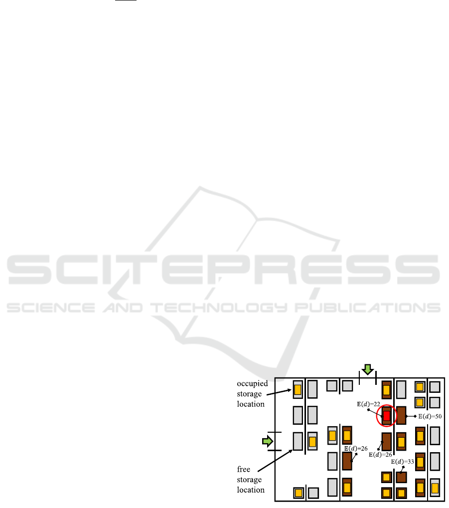
In the second stage of the decision-making, after

having determined a suitable warehouse cluster for

the incoming product in the first stage of the decision-

making, a distance-based decision rule is used to

identify a specific storage location within the target

cluster. Thus, as visualized in Figure 2, the storage

position with the smallest expected distance to the

warehouse exit is selected. In case the action selected

by the agent is infeasible, i.e., in case the desired

warehouse cluster has insufficient storage capacity, a

random available storage location is chosen from the

warehouse.

Figure 2: Representation of the distance-based heuristic

function applied for the allocation of incoming products

(red rectangle) to a specific storage position in the target

spatial cluster.

A Concept for Optimal Warehouse Allocation Using Contextual Multi-Arm Bandits

463

3 CASE STUDY

3.1 Setup

A warehouse comprising a total of 4,650 storage

locations for pallets or small load carriers is consider-

ed. The storage locations are distributed among differ-

ent types of storage systems, that are three pallet racks,

a sliding shelf, a mobile rack, two shelving racks and a

pallet storage. In this case study, 30 different product

types are considered. Synergies among the products are

modelled using six “product clusters”. Each product

cluster contains product types that are more likely to be

part of the same customer order. Customer orders are

generated by a warehouse simulation software, which

first draws the number of products for a certain order

randomly from a set of order sizes 𝑂=



1,2,3,4



Then, the types of products part of the order are

selected based on the “order probability” 𝑃



, defined as

the probability to select products from a certain product

cluster. In this case study, 𝑃



is chosen as 69 % for the

second product cluster and as 6 % for the remaining

five product clusters.

For the spatial clustering, the scikit-learn

implementation of the BIRCH algorithm is applied to

the time matrix 𝑫, representing the distance in terms

of travel time intervals between the different storage

locations. The parameter threshold for the BIRCH

algorithm is chosen as 0.2 and 50 clusters are used.

3.2 Result

3.2.1 Turnover Frequency and Product

Synergy

Before discussing the training results of the agent, the

turnover frequency and product synergy of the

different product types are considered. Recalling

Subsection 2.2.2, both metrics are crucial for the

decision-making of the agent and thus continuously

updated for each product using historical data

recorded throughout the training.

For reference, the mean normalized turnover

frequency of each product cluster after 30,000

training iterations is given in Table 1 and validated

against the settings of the simulation.

As expected when considering the order

probability of the clusters, the second product cluster

has the highest turnover frequency. The products in

the remaining product clusters have significantly

lower turnover frequencies. Note that the different

values in the turnover frequency for the remaining

clusters result from each cluster having a different

number of products.

Table 1: Resulting turnover frequencies for each product

cluster.

Product cluster Mean normalized

turnover frequency

1 0.385

2 0.985

3 0.205

4 0.279

5 0.073

6 0.504

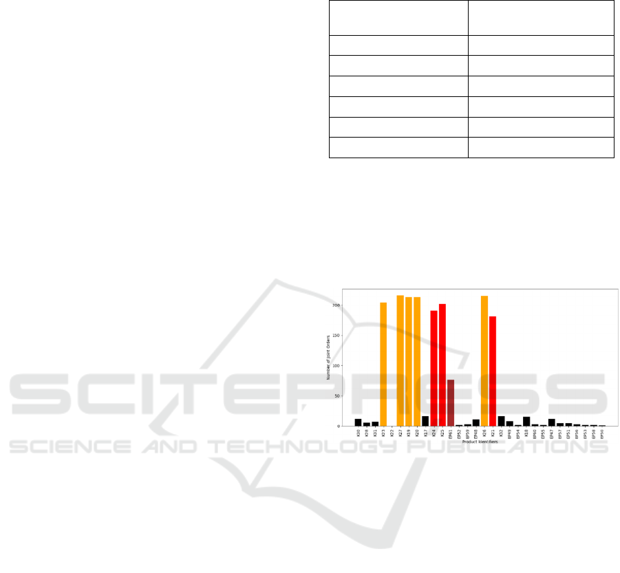
Additionally, the result of the synergy analysis

after 30,000 iterations is demonstrated for the

exemplary product type “K21”. The synergy is

expressed by the number of joint orders of this

product type with any of the remaining 29 product

types. A bar plot representation of the product

synergy is visualized in Figure 3.

Figure 3: Example of order synergy of a product in product

cluster 2. Products of synergy class 0 are displayed in black,

those of synergy class 1 in dark red, those of synergy class

2 in red, and those of synergy class 3 in orange.

Depending on the relative number of joint orders,

each product type is classified into one of four

synergy classes. The synergy classes are visualized in

Figure 3 using colour. Note that the categorization of

each product type may substantially differ depending

on the product type for which the joint synergy is

considered.

3.2.2 Learning Curve

Figure 4 visualizes the performance of the agent

throughout the course of the training. The learning

curve shows a clear increase in the attained reward.

After 𝟏.𝟐𝟎 𝒙

𝟏𝟎

𝟒

training iterations, a mean reward

of 0.85 is reached. Moreover, the infeasibility

percentage, i.e., the ratio with which the agent makes

infeasible storage suggestions, decreases to 0.03 %.

These results demonstrate that the LinUCB agent is

able to identify a storage allocation strategy that

ICEIS 2023 - 25th International Conference on Enterprise Information Systems

464

reaches elevated positive rewards by selecting

feasible storage positions that are optimal in terms of

product synergy, turnover frequency, and the

expected distance to the warehouse exit.

To validate the performance of the LinUCB agent

the learned storage allocation policy is compared to

that of a conventional ABC-analysis-based allocation

strategy. To this end, based on their normalized

turnover frequency, all product types are categorized

as A-, B-, or C-type products. If a product has a

normalized turnover frequency higher than 80 %, the

product is of A-type; if it is between 80 % and 20 %,

the product is of B-type; all other products are C-type.

Additionally, each storage position in the warehouse

is categorized by industry experts as either A-, B-, or

C-type. The ABC-analysis-based allocation strategy

then positions A-type products in A-type spatial

clusters, B-type products in B-type spatial clusters,

and so on. If there are more spatial clusters belonging

to the same type, priority is given to the cluster that

has the smallest expected distance to the warehouse

exit.

In the following, the decision-making of the

LinUCB agent is evaluated using two storage

allocation examples. In both cases, there is about 30

% remaining capacity of the warehouse.

Figure 4: Results of the learning process of the LinUCB

agent over 2.25 𝑥 10



iterations.

3.2.3 An Exemplary Storage Allocation for

an a-Type Product

First, we consider the storage allocation suggestion of

the LinUCB agent for an incoming product of product

type “K20". This product has a normalized turnover

frequency of 0.985 (A-type) and thus constitutes one

of the most frequently ordered product types. The

action valuation of the LinUCB agent for a subset of

the 50 spatial clusters is shown in Figure 5. In the first

column, the normalized expected distance of each

cluster is shown.

Figure 5: Example of the action valuation of the LinUCB

Agent for the A-type product “K20”.

Moreover, information about the remaining

capacity of each cluster is provided in the second

column. Information about the product synergy is

given in the remaining columns. Specifically, each

column gives the percentage of synergy class

products, ordered from synergy class 0 to synergy

class 3 from left to right, that are located in each

cluster.

In this particular example, the agent indicates

cluster 18 as the best allocation target. This decision

is reasonable, given the low expected distance to the

warehouse exit, the sufficient feasibility, and the high

product synergy of “K20” with products already

stored in this spatial cluster, as indicated by the high

product synergy scores.

As the second-best choice, the agent indicates

cluster 10, which has the same expected distance to

the warehouse exit as cluster 18. Note that cluster 10

has a considerably higher product synergy than

cluster 18. However, its remaining storage capacity is

smaller than that of cluster 18, although it would

suffice to store product “K20”. This raises the

question why the LinUCB agent still prefers cluster

18 over cluster 10? The reason for this is that the

agent experienced during training that the selection of

a cluster with zero capacity leads to a negative

reward. It thus learned a linear dependence between

the received reward and the remaining storage

capacity of the selected cluster. Therefore, the

LinUCB agent associates clusters having low

remaining storage capacity with a higher probability

to receive a negative reward.

Cluster 25 constitutes the lowest valued option.

This is once again reasonable, considering that this

cluster has neither sufficient remaining storage

capacity nor existing product synergies.

The conventional ABC-analysis-based allocation

strategy suggests to store product “K20” in cluster 10.

The second and third best choices are clusters 18 and

49. Note that the LinUCB agent considers cluster 49

as the fifth best choice. These results indicate that the

suggestions of the LinUCB agent match those of the

A Concept for Optimal Warehouse Allocation Using Contextual Multi-Arm Bandits

465

conventional allocation strategy. In other words, it

appears that the agent learned a valid storage

allocation strategy.

3.2.4 An Exemplary Storage Allocation for a

B-Type Product

Next, the storage suggestion of the LinUCB agent for

an incoming product of type “K17” with normalized

turnover frequency of 0.385 (B-type) is considered.

The action valuation of the LinUCB agent for a subset

of the 50 spatial clusters is shown in Figure 6.

Figure 6: Example of the action valuation of the LinUCB

Agent for the B-type product “K17”.

The LinUCB agent suggests to store the product

in cluster 18. This is because cluster 18 has a low

expected distance, sufficient capacity, and a high

product synergy. Specifically, 10 % of the products

already stored in cluster 18 are product types that

have the highest synergy level with “K17”.

This time, the suggestion of the conventional

ABC-analysis based allocation strategy differs from

that of the LinUCB agent. The conventional strategy

suggests clusters 38 or 3 as best choices, i.e., two B-

type clusters with low expected distance to the

warehouse exit.

This discrepancy in the decision-making

highlights a main deficiency of the ABC-based

strategy: synergy effects between different ABC-

types of products are not considered. In contrast, the

LinUCB agent suggests to store the B-type product

“K17” in cluster 18, that is a cluster containing a

majority of A-type products. This is because “K17”

synergizes with those A-type products. This

demonstrates that, because of the reward function, the

LinUCB agent is able to consider inter-categorical

product synergy effects in its decision-making

process.

4 CONCLUSIONS

This paper applies a LinUCB agent to identify

optimal storage locations for incoming products in

logistic warehouses. The main contributions are as

follows:

• Demonstration of good learning results for the

LinUCB agent after only 1.20 x 10



training

iterations, reaching an average reward of 0.85

and a percentage of infeasible actions of only

0.03 %.

• The capacity of the LinUCB agent to base its

decision on turnover frequency, expected

distance to the warehouse exit, and product

synergy effects.

• Demonstration that the performance of the

LinUCB agent matches that of a conventional

ABC-analysis based storage allocation

strategy. In contrast to the conventional

method, the agent also considerers inter-

categorical product synergies in the decision

making.

It is to be noted that, the reward function used in

this paper replaces the true picking cost, which – at

the time of the decision-making lies in the future – by

a heuristic metric based on information about product

synergy, travel distance, and available storage

capacity. To minimize the risk of biasing the

decision-making of the agent, future research is

required to design, implement, and test an alternative

reward function – or “delayed” reward – design that

does rely on significantly less heuristic domain

knowledge.

FUNDING

This research has been leaded in the context of the

Zentrales Innovationsprogramm Mittelstand [Central

Innovation Programme for SMEs] (ZIM) project “

SeSoGEN: Entwicklung einer selbstlernenden

Software zur Generierung intelligenter

Einlagerungsstrategien auf Basis neuronaler Netze”.

The Federal Ministry for Economic Affairs and

Energy, based on a decision of the German Bundestag

[Federal Parliament], funded this project.

ACKNOWLEDGEMENTS

We would like to thank Andreas Engelmayer,

Hannelore Mayr, Gertrud Contardo, Markus

Proschmann from the firm CIM GmbH for the fruitful

collaboration. Specifically, CIM GmbH provided the

time matrix 𝑫 , categorized the storage locations

according to the conventional ABC-analysis, and

ICEIS 2023 - 25th International Conference on Enterprise Information Systems

466

used the software PROLAG World to simulate

incoming products, warehouse state and customer

orders.

The authors wish it to be known that, in their

opinion, the first two authors should be regarded as

joint first authors.

REFERENCES

De Koster, R., Le-Duc, T., Roodbergen, K. J. (2007).

Design and control of warehouse order picking: A

literature review. In European Journal of Operations

Research 182.2, pp. 481-501.

Heragu, S. S., Du, L., Mantel, R. J., Schuur, P. C. (2005)

Mathematical model for warehouse design and product

allocation. In International Journal of Production

Research 43:2, pp. 327−338.

Jiao, Y., Xing, X., Zhang, P., Xu, L., Liu, X−R. (2018).

Multi−objective storage location allocation

optimization and simulation analysis of automated

warehouse based on multi−population genetic

algorithm. In Concurrent Engineering Research and

Applications 26:4, pp. 367−377.

Li, L., Chu, W., Langford, J., Schapire, R. E. (2010). A

contextual-bandit approach to personalized news article

recommendation. In Proceedings of the 19

international conference on World wide web – WWW

’10. ACM Press.

Petersen, C. G., Aase, G. (2004). A comparison of picking,

storage and routing policies in manual order picking. In

International Journal of Production Economics 92.1,

pp. 11-19.

Rushton, A., Croucher, P., Baker, P., Transport, C. (2010).

The Handbook of Logistics and Distribution

Management. Kogan Page.

Zhang, T., Ramakrishnan, R., Livny, M. (1996). BIRCH:

An Efficient Data Clustering Method for Very Large

Databases. In SIGMOD Rec. 25.2, pp-103-114.

A Concept for Optimal Warehouse Allocation Using Contextual Multi-Arm Bandits

467