Predictive Power of Two Data Flow Metrics in Software Defect Prediction

Adam Roman

, Rafał Bro

zek and Jarosław Hryszko

Jagiellonian University, Faculty of Mathematics and Computer Science, Poland

Keywords:

Software Defect Prediction, Data Flow Metrics, Dep-Degree, Data Flow Complexity, Within-Project Defect

Prediction.

Abstract:

Data ﬂow coverage criteria are widely used in software testing, but there is almost no research on low-level

data ﬂow metrics as software defect predictors. Aims: We examine two such metrics in this context: dep-

degree (DD) proposed by Beyer and Fararooy and a new data ﬂow metric called dep-degree density (DDD).

Method: We investigate the importance of DD and DDD in SDP models. We perform a correlation analysis

to check if DD and DDD measure different aspects of the code than the well-known size, complexity, and

documentation metrics. Finally, we perform experiments with ﬁve different classiﬁers on nine projects from

the Uniﬁed Bug Dataset to compare the performance of the SDP models trained with and without data ﬂow

metrics. Results: 1) DD is noticeably correlated with many other code metrics, but DDD is not correlated or

is very weakly correlated with other metrics considered in this study; 2) both DD and DDD are highly ranked

in the feature importance analysis; 3) SDP models that use DD and DDD perform better than models that do

not use data ﬂow metrics. Conclusions: Data-ﬂow metrics: DD and DDD can be valuable predictors in SDP

models.

1 INTRODUCTION

Software defect prediction (SDP) is a widely in-

vestigated research area in software engineering.

Many different SDP models were proposed, includ-

ing within-project, cross-project, and just-in-time de-

fect prediction (Kamei et al., 2013; Shen and Chen,

2020). Recent advances in the ﬁeld focus on deep

learning techniques and use different semantic repre-

sentations of programs based on a given set of fea-

tures, such as token vectors extracted from programs’

Abstract Syntax Trees (Mikolov et al., 2013; Zhang

et al., 2019; Shi et al., 2020). Another approach is

to use the so-called hand-crafted features deﬁned by

experts. They characterize the statistical properties

of the code, such as program size, complexity, code

churn, or process metrics.

In modern approaches, extracting implicit struc-

tural, syntax, and semantic features from the source

code is preferred over using explicit hand-crafted ones

(Akimova et al., 2021). However, the classical code

metrics should not be underestimated. First, con-

trary to the semantic features, hand-crafted features

describe structural code complexity, which comple-

ments the semantic view. Second, classical code met-

https://orcid.org/0000-0002-1020-5128

rics are simple and easy to understand by a human.

The models that use them are better explainable than

models that use, for example, deep neural networks

based on token vectors that have no meaning to the

developer. Third, one of the key factors contributing

to the difﬁculty of the SDP is the lack of context. As

pointed out in (Akimova et al., 2021), unlike natural

texts, the code element may depend on another ele-

ment located far away, maybe even in another class,

ﬁle, or component. Therefore, a simple metric that

captures such relations could be very helpful as an

additional feature in SDP models (for example, data

ﬂow metrics are widely used in automatic software

vulnerability detection (Shen and Chen, 2020)).

Interest in data ﬂow metrics comes from the hy-

pothesis that defect proneness depends not only on

the project structure or program semantics but also

on the complexity of information ﬂow that occurs in

a module or system. Miller’s hypothesis on the ca-

pacity to process information (Miller, 1956) suggests

that the more dependencies a program operation has,

the more different program states must be considered

and the more difﬁcult it is to understand the operation.

When a developer writes or modiﬁes a given line of

code, there is a higher chance of error and of introduc-

ing a defect if the variables used in this line depend on

more other places in the code.

114

Roman, A., Bro

zek, R. and Hryszko, J.

Predictive Power of Two Data Flow Metrics in Software Defect Prediction.

DOI: 10.5220/0011842200003464

In Proceedings of the 18th International Conference on Evaluation of Novel Approaches to Software Engineering (ENASE 2023), pages 114-125

ISBN: 978-989-758-647-7; ISSN: 2184-4895

 2023 by SCITEPRESS – Science and Technology Publications, Lda. Under CC license (CC BY-NC-ND 4.0)

Research on data ﬂow is still quite intensive in

data ﬂow testing, regarding the test coverage crite-

ria, like all-defs, all-uses, all-du-paths, etc. (Am-

mann and Offutt, 2016; Hellhake et al., 2019; Neto

et al., 2021; Kolchin et al., 2021). However, it does

not seem to attract much attention from researchers

in the context of SDP models. For example, popular

bug databases like PROMISE (Sayyad Shirabad and

Menzies, 2005), Eclipse (Zimmermann et al., 2007),

GitHub Bug Dataset (Ferenc et al., 2020) use many

different metrics, but none of them uses any kind of

metric related to low-level data ﬂow complexity, such

as number of du-paths in the source code.

Therefore, it is not surprising that studies of SDP

models also rarely use data ﬂow metrics as indepen-

dent variables. For example, just-in-time prediction

models focus almost exclusively on process metrics

(Kamei et al., 2013; Rahman and Devanbu, 2013).

The most popular data ﬂow-related concepts used in

SDP research are some coarser features, like fan-

in and fan-out, calculated at the method level. In

their survey article,

Ozakıncı and Tarhan (

Ozakıncı

and Tarhan, 2018) refer to several SDP models and

note that the only metric related to the data ﬂow

used in them is the ’data ﬂow complexity’ (Pandey

and Goyal, 2009, 2013; Kumar and Yadav, 2017) de-

ﬁned by Henry and Kafura (Henry and Kafura, 1981),

based on the above-mentioned features. The new pa-

pers focus mainly on deep learning methods and seem

to disregard the concept of data ﬂow. For example,

(Shi et al., 2020) uses Code2vec (Alon et al., 2019)

– one of the best source code representation models,

which takes advantage of deep learning to learn au-

tomatic representations from code. One of the code

characteristics used in (Shi et al., 2020) is the concept

of path, but not related to data ﬂow paths.

In 2010, a new data ﬂow metric, called dep-degree

(DD), was proposed (Beyer and Fararooy, 2010). The

idea is to quantitatively describe the concept of so-

called du-paths by counting the number of pairs (p,q)

of nodes in the data ﬂow graph for which there exists

a path on which some variable is deﬁned in p, used

in q, and not redeﬁned in between. This metric can

be viewed as a more detailed version of the Oviedo

metric, because it is based on the source code instruc-

tions, not on the basic blocks of code.

Akimova claims that hand-crafted features, like

all above-mentioned data ﬂow metrics, usually do not

sufﬁciently capture the syntax and semantics of the

source code: ’Most traditional code metrics cannot

distinguish code fragments if these fragments have

the same structure and complexity, but implement a

different functionality. For example, if we switch sev-

eral lines in the code fragment, traditional features,

such as the number of lines of code, number of func-

tion calls, and number of tokens, would remain the

same. Therefore, semantic information is more im-

portant for defect prediction than these metrics’ (Aki-

mova et al., 2021).

However, there are at least three substantial rea-

sons suggesting that DD can be a good defect predic-

tor in the SDP models:

• DD correlates well with the developer’s subjective

sense of ’difﬁculty’ to understand a source code

(Katzmarski and Koschke, 2012),

• the same correlation was observed by direct mea-

surement of developers’ brain activity using fMRI

(Peitek et al., 2020),

• DD is the only known metric that satisﬁes all nine

Weyuker properties (Weyuker, 1988; Beyer and

aring, 2014).

The last reason is also the answer to Akimova’s

objection: it is true that metrics like lines of code

or cyclomatic complexity do not distinguish the pro-

grams in which several lines of code were switched.

However, one of the Weyuker properties of a well-

designed metric requires exactly that there exist at

least two programs, where one is created from the

other by permuting some lines, and the metric is dif-

ferent for these two programs. The DD metric, in

particular, fulﬁlls this condition (Beyer and H

aring,

2014).

Since, to our best knowledge, there is no research

on DD regarding the SDP models, the natural next

research steps are to verify if the data ﬂow metrics

are redundant with other classical source code metrics

and to measure the importance of data ﬂow metrics in

such models. Apart from DD, in our research we will

also investigate its composite variant proposed by us –

dep-degree density (DDD), understood as DD divided

by the number of logical lines of code. The justiﬁca-

tion for introducing this metric is given in Section 2.

Now we can formally state three research ques-

tions that we answer in this paper.

RQ1. Do the DD and DDD metrics measure the same

aspects of the source code as other classical

source code metrics?

RQ2. What is the importance of DD and DDD as fea-

tures in SDP models?

RQ3. How does the use of DD and DDD affect the

performance of the model?

Although there are models that predict the actual

number of residual defects, in this paper we consider

classiﬁcation models, which are the most common ap-

proach to defect prediction (Akimova et al., 2021). In

Predictive Power of Two Data Flow Metrics in Software Defect Prediction

115

these models, a prediction for a given source code ele-

ment is ’yes’ (if the model predicts at least one defect

in the code) or ’no’ otherwise.

The paper is organized as follows. In Section 2 we

formally deﬁne the DD and the DDD proposed by us.

In Section 3 we describe the results of experiments

that answer the research questions RQ1–RQ3 about

the correlation, importance of features, and predictive

power of DD and DDD. Section 4 presents the threats

to validity in our study. A discussion of the results

and possible future research follows in Section 5.

2 DATA FLOW METRICS

To formally introduce the deﬁnition of DD, we need

to deﬁne a data ﬂow graph (DFG), a model built on

the concept of a control ﬂow graph, enriched with in-

formation on where the deﬁnitions and uses of vari-

ables occur. A control ﬂow graph G = (S,E) is a di-

rected graph, where S represents program operations,

and E ⊆S ×S is a set of control ﬂow edges of the pro-

gram. A program operation may be either a variable

declaration, an assignment operation, a conditional

statement, a function call, or a function return. A path

of length k in G is a sequence of nodes (s

,..., s

) such

that (∀i ∈ {0,...,k −1}) (s

i+1

) ∈ E.

Program operations read and write values from/to

variables. Each place in which a value of a variable

v is stored into memory (because of deﬁning or com-

puting the variable’s value) is called a deﬁnition of S.

Each place in which a value of a variable v is read

from memory is called a use of v.

Let V be the set of all variables (attributes and ob-

jects) of a given program P represented by a control

ﬂow graph G = (S, E). A data ﬂow graph for G is a tu-

ple D

= (S,E,de f ,use), where de f ,use : S →V are

functions that store information about the deﬁnitions

and uses of variables in different program operations:

• (∀v ∈V )(∀s ∈ S) v ∈ de f (s) ⇔ v is deﬁned in s;

• (∀v ∈V )(∀s ∈ S) v ∈ use(s) ⇔ v is used in s.

A path p = (s

,..., s

) in D

is called a du-path for

v ∈V , if the following conditions are satisﬁed:

• v ∈de f (s

• v ∈use(s

• (∀1 ≤i ≤ k −1) v ̸∈ de f (s

In other words, v is deﬁned in s

, used in s

, and

there is no redeﬁnition of v along p. Dep-degree met-

ric (DD) is deﬁned as the number of pairs (s, s

′

) of

operations such that there exists a du-path from s to

′

for some variable v. Originally, DD was deﬁned

in terms of the number of nodes’ out-degrees in a so-

called dependency graph (Beyer and Fararooy, 2010).

However, assuming that each operation contains at

most one deﬁnition, we can reduce it to the prob-

lem of counting the du-paths in the code and deﬁne

it as follows. Let G = (S,E) be a control ﬂow graph

with a set V of variables, and let v ∈ V,s,s

′

∈ S. Let

dup(v,s,s

′

) = 1 iff there exists a du-path from s to s

′

for v; otherwise, dup(v,s,s

′

) = 0. Then

DD(D

) =

∑

v∈V

∑

s∈S

∑

′

∈S

dup(v,s,s

′

Beyer and Fararooy (Beyer and Fararooy, 2010)

compare DD with two classical metrics: lines of code

and cyclomatic complexity. They give several exam-

ples of pairs of programs with the same value of these

two metrics, but differing in DD value, showing that

DD is a good indicator of readability and understand-

ability.

However, the opposite situation may also occur.

DD may be ’insensitive’ to program size. In Fig. 1

two equivalent programs are shown. Both have the

same dep-degree (DD=16), but one is twice as long

(10 LOC) than the other (5 LOC). The code on the

left may be considered easier to understand because

its lines contain simpler computations. However, this

comes at the expense of more variables, deﬁnitions,

and lines of code. The right program has fewer deﬁ-

nitions and is shorter, but this makes it more ’dense,’

which may cause more difﬁculties for a programmer

to understand it, and hence makes it more error-prone.

It is easy to provide a similar example in the case

of cyclomatic complexity, showing the possible insen-

sitivity of DD to program structural complexity. Two

programs can have the same DD but differ in cyclo-

matic complexity.

To grasp the concept of data ﬂow ’density’ we

introduce a new metric called dep-degree density

(DDD). It is deﬁned as the value of DD divided by

the logical lines of code: DDD = DD/LLOC. Since

we consider code metrics on the class level, by LLOC

we understand the number of non-empty and non-

comment code lines of the class, including the non-

empty and non-comment code lines of its local meth-

ods, anonymous, local, and nested classes (to measure

it we use the TLLOC metric from Open Static Ana-

lyzer).

3 EXPERIMENTS

In this section we present the experimental results on

investigating the correlation, feature importance, and

predictive power of DD and DDD metrics in the SDP

models.

ENASE 2023 - 18th International Conference on Evaluation of Novel Approaches to Software Engineering

116

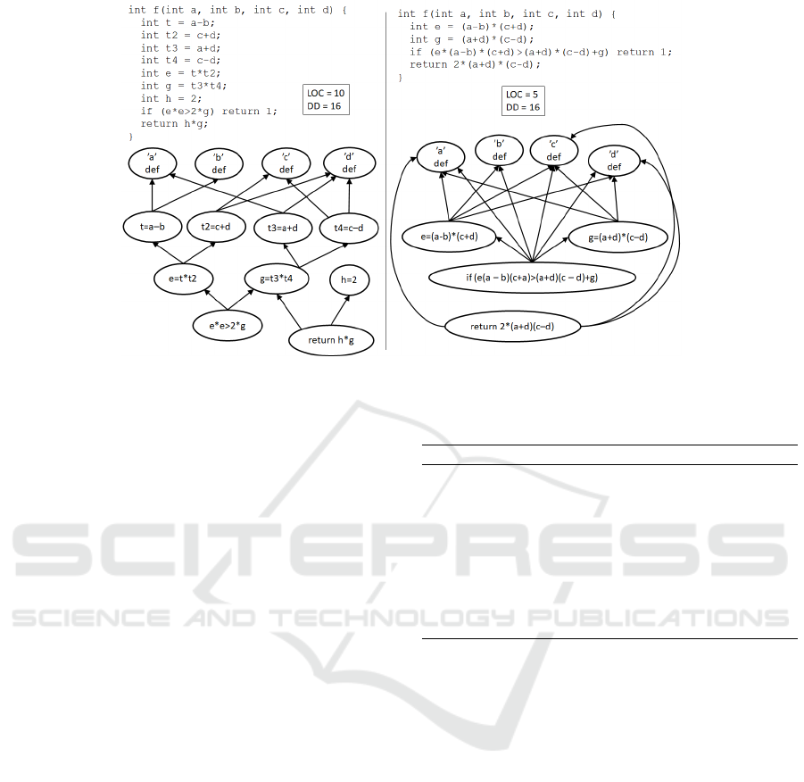
Figure 1: Two equivalent programs with the same DD but different LOC.

Notice that in this research we do not intend to in-

vestigate relations between metrics, examine the in-

ﬂuence of a given resampling method in the train-

ing process, choose the best possible set of metrics,

ﬁnd the best possible SDP model in terms of different

performance measures, compare the models obtained

with other models from the literature, etc. Our inten-

tion is only to verify if DD and DDD metrics can be

useful in defect prediction, that is, if they have a pos-

itive inﬂuence on the SDP model performance. Other

aims mentioned above are an important but separate

issue, out of the scope of this research. Since DD and

DDD are static code metrics, we compare them with

other such metrics, not with process metrics or prod-

uct metrics.

3.1 Datasets and Metrics Used

For our experiments, we selected bug data from

nine JAVA projects from the GitHub Bug Dataset.

The data are part of the Uniﬁed Bug Dataset

(Ferenc et al., 2020). The overview of the se-

lected projects is shown in Table 1. Each ﬁle

is described with a set of 62 metrics measured

by the Open Static Analyzer (github.com/sed-inf-u-

szeged/OpenStaticAnalyzer). 52 of them are class-

level metrics (incl. 4 complexity metrics, 5 coupling

metrics, 8 documentation metrics, 5 inheritance met-

rics, 30 size metrics), 9 are code duplication metrics,

and one (cyclomatic complexity) is a complexity met-

ric computed at the ﬁle level. For detailed deﬁnitions

of these metrics, see the Open Static Analyzer docu-

mentation.

For each ﬁle in the database, we added two data

ﬂow metrics described above: DD and DDD. DD was

Table 1: Overview of the selected projects. kLLOC = size

in kilo Logical Lines of Code.

Project kLLOC Classes Bug % bug

el elasticsearch 219.4 2781 445 16.0

hz hazelcast 112.5 1809 276 15.3

br broadleaf 59.8 1272 274 21.5

ti titan 57.9 787 66 8.4

ne netty 35.6 732 219 29.9

ce ceylon 78.0 678 55 8.1

or oryx 12.3 263 43 16.3

cm cMMO 11.0 248 57 23.0

md mapdb 35.7 133 20 15.0

measured using the AntLR tool, which returns the ab-

stract syntax tree (AST) of the source code. To cal-

culate DD, we transformed the resulting ASTs into

data ﬂow graphs and measured DD using the classical

iterative technique of computing the data ﬂow equa-

tions (Kennedy, 1979), which allowed us to calculate

the reachability of each variable in each statement of

the source code and count the number of resulting du-

paths.

3.2 Correlation Analysis

Recent studies show that eliminating correlated met-

rics improves the consistency of the rankings pro-

duced and impacts model performance. Thus, when

one wishes to derive a sound interpretation from the

defect models, the correlated metrics must be miti-

gated (Tantithamthavorn et al., 2016; Tantithamtha-

vorn and Hassan, 2018; Jiarpakdee et al., 2021).

Therefore, the natural question arises: Are DD and

DDD correlated with other metrics?

To verify this and to answer RQ1, we used the

Predictive Power of Two Data Flow Metrics in Software Defect Prediction

117

AutoSpearman method (Jiarpakdee et al., 2018), im-

plemented in the R package Rnalytica, with default

parameters (threshold = 0.7, vif = 5), as well as a

direct analysis of the correlation of DD and DDD

with other source code metrics. Correlation analy-

sis allows us to verify whether two metrics measure

the same or different aspects of the source code. A

very high correlation between two metrics m

and m

suggests that they measure similar code characteris-

tics, so it is not necessary to use them both in a SDP

model. In this way, we also reduce the number of vari-

ables without signiﬁcantly reducing the model perfor-

mance. On the other hand, very low correlation sug-

gests that m

and m

measure substantially different

aspects of the code, so both should be included in the

SDP model, increasing its performance.

We applied AutoSpearman to the entire Uniﬁed

Bug Dataset with DD and DDD metrics added. It re-

turned 17 (out of 64) least correlated metrics: CLC,

LCOM5, NLE, CBO, CBOI, AD, PUA, NOC, NLA,

NLG, NLPA, NLS, NPA, NPM, NS and dep-degree

density (DDD). This allows us to claim that DDD

measures different code aspects than other static code

metrics. An interesting fact is that AutoSpearman did

not choose cyclomatic complexity, which is a very

popular complexity metric commonly used in soft-

ware defect prediction models. The reason may be

that it is very highly correlated with other metric re-

turned by AutoSpearman, NLE – Nesting Level Else-

If (correlation 0.82).

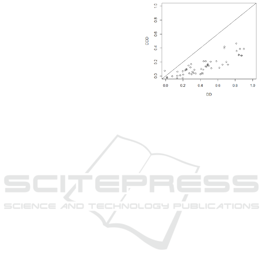
We also investigated the correlation between the

data ﬂow metrics and all other metrics used in this

study. In general, DDD turned out to be very weakly

correlated with all other metrics. The correlation is

also much weaker than in the case of DD. Fig. 2

presents the correlations of DD and DDD with all

other metrics. Each point shows the correlation of

some metric with DD (X-axis) and DDD (Y-axis) ex-

pressed in terms of Pearson correlation coefﬁcient.

Only for seven metrics is the correlation with

DDD greater than 0.3. These are: NL (0.421), NLE

(0.401), TNOS (0.388), NOS (0.388), WMC (0.357),

LLOC (0.302), and LOC (0.300). However, even

for these metrics, the correlation is relatively weak.

For DD, we obtained much stronger correlations. For

eight metrics (McCC, TNOS, TLLOC, TLOC, NOS,

LLOC, LOC, and WMC), the correlation is very high

(between 0.8 and 0.9), for nine metrics (TNLM, RFC,

NL, NLE, NLM, TNLPM, TNLA, NLPM, NLA) be-

tween 0.5 and 0.8, and for 16 others (NOI, CCO,

LLDC, LDC, CI, TCLOC, CLOC, CBO, TNM, PUA,

TNA, TNPM, NM, NATTR, TNLG, LCOM5) it is be-

tween 0.3 and 0.5. The correlation between DD and

DDD is 0.52.

Figure 2: Pearson correlation coefﬁcients for correlation of

DD and DDD with other analyzed metrics.

This analysis answers RQ1: DDD measures as-

pects of the code different from any other metric mea-

sured by the Open Static Analyzer. DD, on the other

hand, is very similar to at least nine other metrics.

3.3 Feature Importance

The importance of features describes how or to what

extent each feature contributes to the prediction of

the model. There are many approaches to measure

it, but the most important features differ depending

on the technique, and a combination of several expla-

nation techniques could provide more reliable results

(Saarela and Jauhiainen, 2021). Therefore, we used

two approaches to calculate the importance of the fea-

tures. The ﬁrst one, the so-called ﬁlter approach, is

model-agnostic. It is based on a ROC curve analysis

for each predictor. The area under the ROC is used

as a measure of variable importance. To perform the

analysis, we used the filterVarImp function from

the caret R package.

The analysis showed that the top ten (out of 64)

features are: McCC (0.73), WMC (0.72), DD (0.70),

TNOS (0.70), TLLOC, TLOC, NL, NLE (0.69), RFC,

and TNLA (0.68). DDD was ranked 23rd (0.63).

In the second approach, we used the built-

in importance measurement mechanism in the

randomForest function. The total decrease in node

impurities from splitting on the variable, averaged

over all trees, is calculated. The node impurity is mea-

sured by the Gini index as follows. For each tree, the

prediction accuracy on the out-of-bag portion of the

data is recorded. Then the same is done after permut-

ing each predictor variable. The difference between

the two accuracies are then averaged over all trees,

and normalized by the standard error. The results are

shown in Fig. 3. DDD and DD metrics were ranked,

ENASE 2023 - 18th International Conference on Evaluation of Novel Approaches to Software Engineering

118

respectively, as 5th (43.7) and 7th (40.8).

From both analyses, it seems that the DD and

DDD metrics are of signiﬁcant importance as defect

predictors, which answers the RQ2. The results of the

second analysis were used in the ’ﬁxed metrics set’

version of the experiment described in the following

(see Section 3.4).

Figure 3: Variable importance – Gini index.

3.4 Experimental Design for the

Within-Project Defect Prediction

Experiment

To investigate the predictive power of data ﬂow met-

rics in the within-project defect prediction setup,

we performed the experiment on the nine above-

mentioned projects with ﬁve SDP models described

below. The experimental design is shown in Fig. 4.

The process described in this ﬁgure was repeated 100

times for each project and model.

Analysis of the distribution of the independent

variables revealed their right skewness. To mitigate

the skew, which introduces different orders of mag-

nitude between variables, we performed the log trans-

formation ln(x+1) for each independent variable (ex-

cept for the density metrics, as they are always scaled

to [0, 1]) as suggested by (Menzies et al., 2007; Jiang

et al., 2008).

The data set is unbalanced – from Table 1 we can

see that the ’bugged’ class accounts for only 8-30%

of all data points. In (Tantithamthavorn et al., 2020),

supported by signiﬁcant empirical data from 101 pro-

prietary and open source projects, the authors argue

that rebalancing techniques are beneﬁcial when the

goal is to increase AUC and recall, but should be

avoided when deriving knowledge and understanding

from defect models. Since our primary goal is to ver-

ify the predictive power of the data ﬂow metrics and

not to build the well-performing SDP models, we in-

tentionally did not use any rebalancing techniques.

The whole experiment was carried out twice, for

two different feature selection strategies. The set of

such selected metrics is denoted by X in Fig. 4. The

ﬁrst strategy uses the sets of non-correlated metrics

selected in each iteration by AutoSpearman. In the

second one, in all iterations we used the ﬁxed set of

ten most important metrics provided by the feature

importance analysis (excluding DD and DDD) per-

formed for the whole data set (see Section 3.3). These

were (see Fig. 3): McCC, WMC, CBO, RFC, NOI,

NOA, TNOS, TLOC, TLLOC and LOC.

In each iteration, the data set was split into train-

ing and test sets in 60%-40% proportions and the fea-

tures (metrics) were selected. We trained ﬁve differ-

ent SDP models: Logistic Regression (LR), Random

Forests (RF), Naive Bayes (NB), k-Nearest Neigh-

bors (KN), and Classiﬁcation and Regression Trees –

CART (CT). The choice was dictated by the fact that

they are widely used by the machine learning com-

munity and have been widely used in many studies

(Bowes et al., 2018). In addition, they are explainable

and have built-in model explanation techniques (Hall

et al., 2012; Tantithamthavorn et al., 2017). More-

over, they use distinct predictive techniques: Naive

Bayes is a generative probabilistic model assuming

conditional independence between variables; logis-

tic regression is a discriminative probabilistic model

that works well also for correlated variables; CART is

an entropy-based model; random forest is an ensem-

ble technique; kNN is a simple, nonparamtric, local,

distance-relying approach. For the hyperparameter

optimization training process, we used the R pack-

age caret and its function train(). We used the

following models implemented in caret: glm, rf,

naive bayes, knn, and rpart.

Each of the ﬁve models was trained in four differ-

ent conﬁgurations:

• using selected metrics only, with no data ﬂow

metrics (X)

• using metrics from X with DD added (DD)

• using metrics from X with DDD added (DDD)

• using metrics from X with both DD and DDD

added (DD+DDD)

In the training process we used the .632 bootstrap,

an enhancement to the out-of-sample bootstrap sam-

pling technique. Recent studies show that out-of-

sample bootstrap validation yields the best balance

between the bias and variance of estimates among

the 12 most commonly adopted model validation

techniques for evaluation. The .632 variant corrects

the downward bias in performance estimates (Efron,

Predictive Power of Two Data Flow Metrics in Software Defect Prediction

119

Figure 4: An overview diagram of the experimental design for our study.

1983; Tantithamthavorn et al., 2017). Using the boot-

strap instead of a simple holdout or cross-validation

approach leverages aspects of statistical inference.

Bowes (Bowes et al., 2018) suggests that re-

searchers should repeat their experiments a sufﬁcient

number of times to avoid the ’ﬂipping’ effect that can

skew prediction performance. The learning process

was therefore repeated 100 times for each combina-

tion of model (5), conﬁguration (4), and project (9).

In each iteration we used different, randomly selected

training and test sets. The model performance met-

rics were then averaged over 100 runs for each of the

5 ×4 ×9 = 180 combinations. This approach miti-

gates the risk of bias in the test data and reduces bias

in the model testing process. Moreover, the split pro-

cedure allowed us to maintain the same defective ratio

in the training and test sets as in the original dataset,

making them representative.

All models were validated on test data and their

performance was compared in terms of F1 score,

ROC-AUC and Matthew’s Correlation Coefﬁcient.

Before we justify the choice of the performance mea-

sures, let us deﬁne them formally. A true positive

(resp. negative) is an outcome when the model cor-

rectly predicts the positive (’bugged’) (resp. negative

(’no bug’)) class. A false positive (resp. negative) is

an outcome when the model incorrectly predicts the

positive (resp. negative) class. Denote by TP, TN, FP,

and FN the number of, respectively, true positive, true

negative, false positive, and false negative outcomes.

F1 Score. Precision is the ratio of TP and all elements

classiﬁed as positive, TP+FP. Recall is the ratio of TP

and the total number of elements belonging to the pos-

itive class, TP+FN. F1 score is the harmonic mean of

precision and recall:

F1 = 2 ×

Precision ×Recall

Precision + Recall

F1 score varies from 0 (no precision or recall) to 1

(perfect classiﬁer).

ROC-AUC. The Area Under the Receiver Operat-

ing Characteristic Curve measures the ability of the

classiﬁers to discriminate between defective and non-

defective examples (Rahman and Devanbu, 2013).

The ROC curve is created by plotting the Precision

against the Recall at various threshold settings. ROC-

AUC is the area under this curve. A perfect classi-

ﬁer has ROC-AUC equal to 1, and a random one has

ROC-AUC = 0.5.

Matthew’s Correlation Coefﬁcient (MCC). MCC is

a measure of association for two binary variables de-

ﬁned as MCC =

T P×T N−FP×FN

√

(T P+FP)(TP+FN)(TN+FP)(TN+FN)

The MCC is a value between −1 (total disagreement

between prediction and observation) and +1 (perfect

classiﬁcation). A classiﬁer with no better prediction

than random has MCC = 0.

F1 is a traditional performance metric, but it is

sensitive to the threshold separating a defective from

a non-defective example. Commonly, this threshold

is conﬁgured to a probability of 0.5. However, this

arbitrary conﬁguration can introduce bias in the per-

formance analysis. ROC-AUC, on the other hand,

is unrestricted to this threshold and provides a sin-

gle scalar value that balances the inﬂuence of preci-

sion (beneﬁt) and recall (cost) (Ma et al., 2012). The

ROC-AUC is also robust to class imbalance, which

is frequently present in software defect prediction

datasets, including the dataset used in this research.

The MCC is a balance-independent metric and com-

bines all quadrants of the binary confusion matrix

(TP, TN, FP, FN), whereas the F1 measure is balance-

sensitive and ignores the proportion of TN. The MCC

has been shown to be a reliable measure of the pre-

dictive performance of the model (Shepperd et al.,

2014) and can be tested for statistical signiﬁcance,

with χ

= N ×MCC

, where N is the total number

ENASE 2023 - 18th International Conference on Evaluation of Novel Approaches to Software Engineering

120

of examples in the data set.

All three measures provide a single value that fa-

cilitates comparison between models. Since different

metrics focus on different aspects of performance, a

proper performance comparison requires the use of

different measures.

3.5 Results of the Within-Project Defect

Prediction Experiment

In the ﬁrst version of the experiment, for each project

and iteration, the set of uncorrelated metrics was se-

lected by AutoSpearman from the set of all metrics,

excluding DD and DDD. Its size ranged from 12

to 19. The most frequently selected metrics were:

LCOM5 (100%), CBO (74%), NOP (73%), NOC,

CBOI, NLA (69%), PUA, NLPA (64%), AD (62%),

CC (53%), NL (50%).

Table 2 presents the results of this experiment.

Notation used: Pr = project name, M = model (see

Section 3.4 for full names), X = models trained with-

out data ﬂow metrics, DD = models trained with

DD added, DDD = models trained with DDD added,

DD+DDD = models trained with DD and DDD

added.

In general (last row of the table summarizing the

results for all projects and classiﬁers), models with no

data ﬂow metrics achieve the worst results in terms

of all three performance measures (F1, ROC-AUC,

MCC). Models using DDD are slightly better, fol-

lowed by those that use DD. Models using both DD

and DDD achieve the best results in terms of all three

performance measures.

It is worth noticing that when allowing

AutoSpearman to choose from the set of met-

rics including the data ﬂow ones, it was always

choosing DDD as one of the non-correlated metrics

and has never indicated DD. However, the experiment

results show that the models using DD perform better

than the models using DDD. This may suggest

that removing correlated metrics does not always

lead us to the best choice of independent variables.

The reason may be that two or more variables

may be highly correlated, but their interaction with

themselves or with other variables may be valuable

information for the model and may signiﬁcantly

impact its performance.

In the second version of the experiment, we used

the ﬁxed set of metrics obtained from the feature im-

portance analysis (see Fig. 3). The results, shown in

Table 3, are similar: models with DD+DDD perform

the best, followed by those that use only one data ﬂow

metric. Models without data ﬂow metrics have the

lowest performance. The results are worse than those

of Table 2, because we used a smaller set of metrics.

For each performance measure we performed the

paired t-test to check the statistical signiﬁcance be-

tween the results of conﬁguration X and the re-

sults obtained for conﬁgurations DD, DDD, and

DD+DDD. The differences turned out to be statisti-

cally signiﬁcant (p < 0.05) in all cases.

This experiment allows us to answer to RQ3 in the

context of within-project SDP: adding the data ﬂow

metrics as the model predictors increases the model’s

performance in terms of all three performance metrics

used.

4 THREATS TO VALIDITY

Construct Validity. The parameters of the learners

inﬂuence the performance of the defect models. The

hyperparameter optimization performed by caret is

done using the train() function, which has its own

parameters, like tuneLength which was always set to

5 in our experiments. This might have had an inﬂu-

ence on the performance results.

Internal Validity. Although it is recommended to

remove correlated variables, it may be the case that

despite the high correlation between two or more

variables, their interaction may be very meaningful

and have a signiﬁcant impact on defect prediction.

We have experienced exactly this phenomenon when

comparing the AutoSpearman results with the per-

formance of the models using DD instead of DDD

(see the discussion in Section 3.5). It is possible

that a feature subset different from the one chosen by

AutoSpearman could affect the performance of the

model and, thus, our results. We mitigated this risk

by performing the second experiment, with a ﬁxed set

of metrics resulting from the feature importance anal-

ysis.

We used 100 repetitions to draw reliable bootstrap

estimates of the performance measures, but this re-

quires a very high computational cost. It may be im-

practical for some compute-intensive ML models or

models that use a large number of independent vari-

ables.

External Validity. Our experiments are based only

on within-project prediction scenarios. We did not in-

vestigate cross-project prediction, just-in-time defect

prediction (Pascarella et al., 2019) or heterogeneous

defect prediction (Nam et al., 2018). The results may

differ in these scenarios, and these models work better

when process metrics are used. In our study we used

static source code metrics only.

We investigated only nine JAVA projects from the

Uniﬁed Bug Dataset. Predictions were made at the

Predictive Power of Two Data Flow Metrics in Software Defect Prediction

121

Table 2: Results of the within-project defect prediction experiment – feature selection done by AutoSpearman in each iteration.

Performance metrics (averaged over 100 runs)

Pr M F1-score ROC-AUC Matthew’s Correlation Coefﬁcient

X DD DDD DD+DDD X DD DDD DD+DDD X DD DDD DD+DDD

CT .634 ± .040 .636 ± .046 .628 ± .042 .630 ± .047 .799 ± .034 .806 ± .031 .798 ± .034 .803 ± .029 .560 ± .046 .560 ± .050 .560 ± .046 .554 ± .051

KN .625 ± .040 .649 ± .041 .624 ± .041 .650 ± .040 .846 ± .021 .855 ± .022 .847 ± .020 .855 ± .020 .553 ± .046 .578 ± .048 .553 ± .046 .579 ± .047

br LR .606 ± .036 .607 ± .037 .608 ± .034 .634 ± .033 .838 ± .023 .838 ± .023 .837 ± .023 .843 ± .023 .535 ± .041 .533 ± .043 .535 ± .041 .563 ± .040

NB .656 ± .037 .668 ± .034 .660 ± .034 .669 ± .034 .849 ± .021 .856 ± .020 .850 ± .021 .856 ± .020 .578 ± .042 .583 ± .041 .578 ± .042 .582 ± .041

RF .683 ± .039 .683 ± .038 .679 ± .038 .682 ± .038 .874 ± .020 .875 ± .019 .875 ± .019 .875 ± .019 .629 ± .042 .629 ± .041 .629 ± .042 .631 ± .040

CT .197 ± .088 .191 ± .082 .192 ± .082 .190 ± .079 .618 ± .069 .612 ± .064 .614 ± .069 .610 ± .066 .174 ± .091 .162 ± .089 .174 ± .091 .162 ± .084

KN .090 ± .022 .108 ± .043 .094 ± .030 .113 ± .046 .721 ± .049 .717 ± .046 .720 ± .052 .712 ± .048 .141 ± .055 .161 ± .063 .141 ± .055 .168 ± .069

ce LR .167 ± .077 .165 ± .075 .167 ± .077 .184 ± .080 .741 ± .045 .737 ± .046 .738 ± .045 .738 ± .045 .187 ± .088 .184 ± .087 .187 ± .088 .202 ± .089

NB .199 ± .070 .215 ± .074 .209 ± .075 .222 ± .076 .750 ± .041 .753 ± .040 .753 ± .041 .754 ± .042 .155 ± .078 .163 ± .084 .155 ± .078 .164 ± .083

RF .125 ± .056 .145 ± .063 .133 ± .056 .146 ± .066 .778 ± .044 .772 ± .046 .775 ± .044 .770 ± .046 .172 ± .077 .201 ± .076 .172 ± .077 .204 ± .081

CT .392 ± .051 .416 ± .050 .388 ± .046 .417 ± .049 .723 ± .038 .753 ± .035 .718 ± .038 .754 ± .035 .346 ± .045 .364 ± .043 .346 ± .045 .364 ± .041

KN .427 ± .039 .437 ± .034 .427 ± .036 .438 ± .035 .826 ± .015 .842 ± .014 .826 ± .015 .842 ± .014 .390 ± .039 .387 ± .035 .390 ± .039 .388 ± .035

el LR .388 ± .030 .392 ± .030 .387 ± .030 .393 ± .030 .822 ± .013 .834 ± .013 .825 ± .013 .834 ± .013 .351 ± .032 .346 ± .031 .351 ± .032 .347 ± .031

NB .308 ± .044 .395 ± .036 .337 ± .042 .410 ± .035

.826 ± .013 .834 ± .012 .827 ± .013 .833 ± .012 .293 ± .039 .351 ± .031 .293 ± .039 .354 ± .033

RF .488 ± .030 .489 ± .028 .473 ± .029 .481 ± .025 .871 ± .011 .879 ± .011 .873 ± .011 .878 ± .011 .460 ± .030 .456 ± .029 .460 ± .030 .450 ± .026

CT .378 ± .056 .382 ± .047 .387 ± .050 .384 ± .048 .695 ± .042 .707 ± .036 .688 ± .042 .706 ± .038 .328 ± .050 .333 ± .042 .328 ± .050 .340 ± .046

KN .401 ± .051 .399 ± .047 .405 ± .051 .406 ± .045 .768 ± .024 .781 ± .024 .767 ± .025 .780 ± .026 .380 ± .042 .372 ± .042 .380 ± .042 .378 ± .041

hz LR .298 ± .038 .322 ± .041 .330 ± .039 .330 ± .039 .772 ± .022 .781 ± .021 .776 ± .021 .779 ± .021 .286 ± .038 .307 ± .041 .286 ± .038 .316 ± .040

NB .391 ± .049 .420 ± .044 .432 ± .045 .449 ± .040 .771 ± .022 .775 ± .022 .775 ± .023 .777 ± .022 .335 ± .046 .348 ± .045 .335 ± .046 .372 ± .043

RF .424 ± .042 .427 ± .041 .418 ± .041 .420 ± .039 .823 ± .020 .825 ± .019 .824 ± .019 .824 ± .019 .411 ± .041 .411 ± .039 .411 ± .041 .408 ± .040

CT .431 ± .104 .420 ± .107 .421 ± .109 .424 ± .109 .718 ± .055 .714 ± .060 .725 ± .059 .722 ± .064 .311 ± .110 .295 ± .114 .311 ± .110 .285 ± .115

KN .349 ± .095 .387 ± .095 .359 ± .098 .390 ± .094 .745 ± .045 .771 ± .045 .747 ± .048 .772 ± .043 .270 ± .095 .303 ± .101 .270 ± .095 .309 ± .096

mc LR .462 ± .074 .492 ± .075 .469 ± .076 .484 ± .082 .781 ± .050 .786 ± .049 .779 ± .049 .786 ± .048 .354 ± .088 .381 ± .090 .354 ± .088 .368 ± .097

NB .458 ± .105 .490 ± .086 .462 ± .101 .506 ± .085 .789 ± .050 .796 ± .047 .798 ± .052 .800 ± .049 .357 ± .111 .376 ± .099 .357 ± .111 .394 ± .101

RF .413 ± .082 .439 ± .087 .428 ± .091 .450 ± .095 .791 ± .046 .797 ± .043 .804 ± .046 .804 ± .044 .322 ± .087 .353 ± .096 .322 ± .087 .371 ± .100

CT .558 ± .139 .559 ± .138 .558 ± .139 .559 ± .138 .787 ± .093 .786 ± .094 .787 ± .093 .786 ± .094 .495 ± .154 .494 ± .154 .495 ± .154 .494 ± .154

KN .562 ± .154 .556 ± .170 .556 ± .156 .568 ± .157 .866 ± .066 .855 ± .065 .863 ± .072 .855 ± .065 .533 ± .149 .527 ± .162 .533 ± .149 .540 ± .151

md LR .493 ± .150 .503 ± .133 .505 ± .139 .517 ± .132 .748 ± .112 .747 ± .104 .756 ± .106 .758 ± .093 .417 ± .169 .424 ± .157 .417 ± .169 .433 ± .160

NB .596 ± .116 .604 ± .117 .592 ± .114 .596 ± .112 .813 ± .083 .826 ± .080 .814 ± .079 .823 ± .077 .534 ± .137 .541 ± .142 .534 ± .137 .532 ± .134

RF .519 ± .160 .523 ± .156 .504 ± .161 .509 ± .168 .889 ± .053 .889 ± .054 .883 ± .058 .887 ± .054 .493 ± .145 .499 ± .146 .493 ± .145 .488 ± .154

CT .601 ± .052 .598 ± .048 .597 ± .056 .594 ± .047 .790 ± .036 .787 ± .035 .787 ± .036 .786 ± .033 .456 ± .062 .450 ± .060 .456 ± .062 .445 ± .059

KN .675 ± .038 .657 ± .037 .675 ± .041 .658 ± .037 .861 ± .021 .854 ± .022 .862 ± .022 .854 ± .022 .540 ± .051 .516 ± .052 .540 ± .051 .517 ± .052

ne LR .494 ± .043 .494 ± .042 .496 ± .043 .492 ± .041 .782 ± .020 .784 ± .021 .783 ± .021 .783 ± .021 .345 ± .053 .344 ± .053 .345 ± .053 .342 ± .052

NB .514 ± .062 .534 ± .054 .532 ± .056 .545 ± .050 .812 ± .022 .807 ± .023 .815 ± .022 .810 ± .024 .371 ± .053 .385 ± .049 .371 ± .053 .393 ± .049

RF .689 ± .045 .685 ± .043 .689 ± .043 .682 ± .043 .899 ± .016 .897 ± .017 .900 ± .018 .896 ± .018 .581 ± .054 .577 ± .051 .581 ± .054 .574 ± .052

CT .406 ± .108 .413 ± .111 .407 ± .114 .408 ± .117 .678 ± .077 .679 ± .078 .682 ± .081 .680 ± .081 .336 ± .124 .338 ± .129 .336 ± .124 .331 ± .132

KN .580 ± .101 .594 ± .089 .580 ± .096 .600 ± .088 .864 ± .049 .865 ± .048 .866 ± .048 .867 ± .044 .529 ± .106 .550 ± .096 .529 ± .106 .556 ± .094

or LR .534 ± .091 .537 ± .094 .534 ± .081 .541 ± .084

.843 ± .049 .840 ± .049 .841 ± .049 .843 ± .049 .462 ± .103 .464 ± .106 .462 ± .103 .467 ± .094

NB .399 ± .151 .413 ± .148 .425 ± .156 .442 ± .150 .830 ± .039 .842 ± .037 .850 ± .035 .854 ± .036 .367 ± .148 .388 ± .138 .367 ± .148 .416 ± .141

RF .570 ± .090 .570 ± .083 .565 ± .093 .554 ± .096 .879 ± .042 .883 ± .041 .883 ± .042 .886 ± .040 .537 ± .095 .545 ± .085 .537 ± .095 .532 ± .096

CT .349 ± .094 .349 ± .093 .344 ± .091 .345 ± .089 .711 ± .058 .714 ± .056 .713 ± .062 .712 ± .062 .335 ± .097 .336 ± .094 .335 ± .097 .331 ± .092

KN .416 ± .075 .431 ± .086 .416 ± .077 .430 ± .084 .772 ± .047 .769 ± .049 .771 ± .049 .772 ± .049 .401 ± .081 .422 ± .092 .401 ± .081 .420 ± .090

ti LR .297 ± .083 .298 ± .080 .294 ± .085 .292 ± .089 .816 ± .043 .814 ± .045 .818 ± .043 .815 ± .043 .279 ± .083 .282 ± .082 .279 ± .083 .272 ± .090

NB .209 ± .108 .226 ± .114 .221 ± .102 .229 ± .101 .743 ± .071 .743 ± .070 .743 ± .070 .742 ± .067 .195 ± .110 .200 ± .118 .195 ± .110 .195 ± .100

RF .456 ± .083 .431 ± .088 .425 ± .081 .405 ± .085 .831 ± .039 .828 ± .040 .827 ± .040 .824 ± .043 .496 ± .072 .474 ± .076 .496 ± .072 .454 ± .072

all .442 ± .172 .452 ± .168 .445 ± .169 .455 ± .167 .794 ± .076 .798 ± .076 .796 ± .077 .799 ± .076 .391 ± .154 .398 ± .151 .391 ± .154 .400 ± .150

ENASE 2023 - 18th International Conference on Evaluation of Novel Approaches to Software Engineering

122

Table 3: Results of the within-project defect prediction experiment – feature set ﬁxed based on feature importance analysis.

Performance metrics (averaged over 100 runs)

Pr M F1-score ROC-AUC Matthew’s Correlation Coefﬁcient

X DD DDD DD+DDD X DD DDD DD+DDD X DD DDD DD+DDD

br CT .612 ± .056 .605 ± .057 .606 ± .052 .604 ± .048 .816 ± .022 .816 ± .023 .814 ± .025 .814 ± .026 .537 ± .047 .529 ± .052 .537 ± .047 .535 ± .047

KN .185 ± .057 .190 ± .058 .187 ± .056 .197 ± .057 .688 ± .059 .688 ± .060 .690 ± .057 .690 ± .062 .192 ± .056 .197 ± .057 .192 ± .056 .202 ± .053

LR .675 ± .028 .675 ± .028 .678 ± .029 .680 ± .029 .871 ± .018 .870 ± .018 .871 ± .019 .871 ± .018 .608 ± .032 .608 ± .032 .608 ± .032 .612 ± .034

NB .576 ± .020 .566 ± .018 .576 ± .020 .565 ± .018 .817 ± .020 .816 ± .019 .823 ± .019 .822 ± .019 .452 ± .029 .440 ± .026 .452 ± .029 .439 ± .026

RF .673 ± .031 .676 ± .032 .673 ± .035 .673 ± .032 .870 ± .015 .875 ± .015 .875 ± .015 .878 ± .015 .617 ± .035 .622 ± .036 .617 ± .035 .621 ± .035

ce CT .168 ± .076 .175 ± .083 .180 ± .080 .183 ± .082 .623 ± .068 .627 ± .066 .622 ± .066 .624 ± .067 .130 ± .081 .136 ± .087 .130 ± .081 .145 ± .092

KN .112 ± .047 .126 ± .049 .111 ± .044 .124 ± .048 .711 ± .057 .707 ± .048 .709 ± .057 .710 ± .048 .158 ± .061 .171 ± .062 .158 ± .061 .177 ± .064

LR .133 ± .066 .141 ± .063 .152 ± .060 .176 ± .065 .741 ± .040 .741 ± .041 .745 ± .042 .744 ± .042 .162 ± .084 .169 ± .080 .162 ± .084 .212 ± .080

NB .251 ± .039 .248 ± .040 .256 ± .042 .252 ± .039 .749 ± .039 .747 ± .039 .750 ± .040 .748 ± .039 .180 ± .053 .178 ± .055 .180 ± .053 .183 ± .054

RF .128 ± .055 .125 ± .054 .130 ± .052 .138 ± .056 .731 ± .049 .728 ± .049 .733 ± .047 .730 ± .044 .145 ± .066 .151 ± .067 .145 ± .066 .171 ± .067

el CT .334 ± .051 .334 ± .048 .330 ± .056 .329 ± .053 .699 ± .045 .699 ± .043 .696 ± .048 .695 ± .044 .278 ± .043 .277 ± .039 .278 ± .043 .272 ± .044

KN .309 ± .039 .317 ± .038 .308 ± .037 .321 ± .041 .757 ± .017 .756 ± .017 .760 ± .017 .757 ± .017 .261 ± .036 .266 ± .035 .261 ± .036 .271 ± .038

LR .325 ± .031 .327 ± .030 .330 ± .030 .325 ± .030 .802 ± .014 .804 ± .013 .804 ± .013 .804 ± .013 .292 ± .031 .293 ± .028 .292 ± .031 .290 ± .029

NB .403 ± .019 .405 ± .018 .408 ± .019 .407 ± .019

.750 ± .015 .753 ± .015 .753 ± .015 .755 ± .015 .266 ± .026 .269 ± .025 .266 ± .026 .271 ± .026

RF .398 ± .032 .392 ± .031 .393 ± .033 .387 ± .032 .829 ± .013 .831 ± .012 .833 ± .013 .831 ± .013 .356 ± .033 .355 ± .032 .356 ± .033 .352 ± .034

hz CT .335 ± .052 .347 ± .058 .351 ± .058 .348 ± .060 .669 ± .038 .677 ± .038 .665 ± .039 .666 ± .040 .284 ± .044 .293 ± .049 .284 ± .044 .301 ± .050

KN .352 ± .045 .353 ± .042 .357 ± .047 .357 ± .041 .699 ± .024 .726 ± .026 .704 ± .024 .729 ± .025 .328 ± .044 .344 ± .043 .328 ± .044 .349 ± .039

LR .316 ± .039 .325 ± .040 .336 ± .039 .328 ± .038 .742 ± .019 .755 ± .019 .752 ± .019 .753 ± .020 .322 ± .039 .319 ± .041 .322 ± .039 .322 ± .040

NB .406 ± .027 .409 ± .027 .425 ± .029 .426 ± .027 .735 ± .021 .739 ± .021 .743 ± .022 .745 ± .021 .284 ± .034 .286 ± .034 .284 ± .034 .308 ± .035

RF .392 ± .039 .396 ± .040 .394 ± .040 .394 ± .040 .775 ± .017 .784 ± .017 .784 ± .018 .788 ± .018 .355 ± .041 .363 ± .040 .355 ± .041 .362 ± .040

mc CT .424 ± .095 .421 ± .102 .415 ± .107 .411 ± .106 .699 ± .050 .697 ± .050 .700 ± .054 .696 ± .054 .277 ± .111 .272 ± .121 .277 ± .111 .263 ± .119

KN .448 ± .082 .456 ± .079 .446 ± .082 .451 ± .084 .780 ± .040 .776 ± .041 .781 ± .039 .777 ± .040 .326 ± .091 .328 ± .087 .326 ± .091 .323 ± .093

LR .474 ± .086 .461 ± .089 .457 ± .090 .476 ± .084 .791 ± .041 .786 ± .042 .788 ± .041 .784 ± .043 .369 ± .101 .350 ± .103 .369 ± .101 .366 ± .100

NB .528 ± .061 .524 ± .061 .528 ± .057 .519 ± .057 .799 ± .038 .798 ± .038 .803 ± .038 .801 ± .038 .377 ± .084 .369 ± .083 .377 ± .084 .361 ± .079

RF .426 ± .085 .415 ± .080 .432 ± .090 .427 ± .089 .758 ± .044 .757 ± .044 .772 ± .042 .769 ± .044 .303 ± .093 .295 ± .085 .303 ± .093 .308 ± .098

md CT .433 ± .144 .430 ± .141 .433 ± .144 .430 ± .141 .734 ± .097 .732 ± .096 .734 ± .097 .732 ± .096 .353 ± .163 .348 ± .160 .353 ± .163 .348 ± .160

KN .415 ± .148 .398 ± .169 .403 ± .141 .394 ± .155 .813 ± .070 .822 ± .068 .809 ± .073 .825 ± .066 .351 ± .167 .341 ± .194 .351 ± .167 .346 ± .170

LR .524 ± .147 .514 ± .148 .527 ± .135 .517 ± .144 .851 ± .100 .846 ± .103 .839 ± .107 .818 ± .113 .463 ± .156 .448 ± .158 .463 ± .156 .449 ± .161

NB .465 ± .103 .496 ± .097 .485 ± .099 .501 ± .097 .817 ± .079 .827 ± .073 .816 ± .073 .821 ± .074 .361 ± .134 .402 ± .127 .361 ± .134 .411 ± .126

RF .467 ± .150 .466 ± .148 .440 ± .137 .434 ± .141 .833 ± .068 .837 ± .065 .831 ± .070 .833 ± .065 .428 ± .162 .427 ± .158 .428 ± .162 .396 ± .155

ne CT .586 ± .052 .590 ± .050 .583 ± .049 .584 ± .048 .769 ± .043 .772 ± .043 .758 ± .043 .762 ± .042 .430 ± .059 .433 ± .059 .430 ± .059 .431 ± .054

KN .605 ± .030 .615 ± .033 .608 ± .032 .616 ± .035 .809 ± .021 .808 ± .022 .810 ± .020 .808 ± .022 .445 ± .043 .452 ± .047 .445 ± .043 .453 ± .051

LR .468 ± .041 .468 ± .040 .467 ± .042 .466 ± .040 .777 ± .019 .775 ± .019 .775 ± .019 .773 ± .019 .319 ± .048 .318 ± .048 .319 ± .048 .315 ± .049

NB .598 ± .029 .593 ± .030 .603 ± .031 .599 ± .030 .786 ± .023 .781 ± .023 .790 ± .023 .784 ± .024 .396 ± .046 .388 ± .048 .396 ± .046 .397 ± .048

RF .643 ± .040 .637 ± .038 .638 ± .037 .635 ± .037 .869 ± .018 .866 ± .018 .866 ± .018 .863 ± .019 .506 ± .053 .498 ± .049 .506 ± .053 .498 ± .050

or CT .389 ± .112 .395 ± .114 .390 ± .111 .393 ± .112 .677 ± .069 .682 ± .076 .678 ± .067 .686 ± .073 .310 ± .108 .316 ± .111 .310 ± .108 .310 ± .112

KN .376 ± .130 .446 ± .108 .395 ± .120 .446 ± .115 .760 ± .058 .773 ± .058 .763 ± .059 .774 ± .058 .318 ± .121 .382 ± .114 .318 ± .121 .382 ± .123

LR .295 ± .111 .288 ± .110 .312 ± .111 .414 ± .100

.734 ± .059 .728 ± .057 .730 ± .058 .775 ± .050 .254 ± .106 .242 ± .112 .254 ± .106 .355 ± .106

NB .449 ± .068 .447 ± .070 .480 ± .070 .472 ± .072 .780 ± .054 .777 ± .053 .804 ± .054 .797 ± .054 .331 ± .088 .326 ± .094 .331 ± .088 .358 ± .094

RF .470 ± .111 .468 ± .110 .471 ± .107 .465 ± .100 .815 ± .045 .818 ± .049 .827 ± .045 .831 ± .047 .434 ± .111 .442 ± .109 .434 ± .111 .445 ± .098

ti CT .303 ± .100 .302 ± .103 .301 ± .101 .299 ± .103 .690 ± .064 .688 ± .066 .686 ± .066 .686 ± .067 .284 ± .106 .283 ± .107 .284 ± .106 .282 ± .108

KN .377 ± .073 .365 ± .078 .382 ± .070 .365 ± .073 .735 ± .053 .723 ± .051 .730 ± .053 .721 ± .052 .356 ± .080 .341 ± .084 .356 ± .080 .338 ± .079

LR .166 ± .081 .166 ± .080 .177 ± .078 .178 ± .079 .788 ± .044 .785 ± .045 .787 ± .045 .781 ± .047 .177 ± .081 .175 ± .080 .177 ± .081 .185 ± .077

NB .151 ± .050 .164 ± .057 .169 ± .063 .178 ± .056 .719 ± .045 .716 ± .046 .718 ± .044 .713 ± .044 .088 ± .061 .093 ± .069 .088 ± .061 .101 ± .065

RF .315 ± .080 .321 ± .084 .312 ± .091 .296 ± .089 .799 ± .048 .794 ± .051 .798 ± .050 .792 ± .050 .328 ± .078 .333 ± .081 .328 ± .078 .313 ± .082

all .397 ± .167 .399 ± .166 .401 ± .164 .404 ± .162 .766 ± .074 .767 ± .073 .767 ± .074 .768 ± .073 .329 ± .143 .330 ± .143 .329 ± .143 .336 ± .139

Predictive Power of Two Data Flow Metrics in Software Defect Prediction

123

class level. The results may be different for projects of

different sizes, maturity, or written in other languages.

They may also differ when performed at the method

or ﬁle level.

5 CONCLUSIONS AND FUTURE

WORK

In this paper we investigated the predictive power of

two data ﬂow metrics: dep-degree and dep-degree

density. DDD measures different aspects of the code

than other metrics considered, since it is weakly

correlated with other metrics. DD shows signiﬁ-

cantly greater correlations. However, using DDD in

SDP models only slightly increases the model perfor-

mance. On the other hand, DD achieves much better

results, but the best results were achieved for models

that used both DD and DDD as independent variables.

To conclude, DD and DDD seem to be the inter-

esting choice as defect predictors in the SDP mod-

els, as well as the objects of future research regard-

ing SDP. They may also be used as useful code com-

plexity metrics, indicating how difﬁcult the code is to

understand by the developer. It would also be inter-

esting to investigate their predictive power in just-in-

time defect prediction models, which recently gained

a lot of attention from researchers.

Data Availability. The source ﬁles (bug data, R

script, and Open Static Analyzer metrics deﬁni-

tions) can be found at https://github.com/Software-

Engineering-Jagiellonian/DepDegree-ENASE2023.

REFERENCES

Akimova, E., Bersenev, A., Deikov, A., Kobylkin, K.,

Konygin, A., Mezentsev, I., and Misilov, V. (2021). A

survey on software defect prediction using deep learn-

ing. Mathematics, 9:1180.

Alon, U., Zilberstein, M., Levy, O., and Yahav, E. (2019).

Code2vec: Learning distributed representations of

code. Proc. ACM Program. Lang., 3(POPL).

Ammann, P. and Offutt, J. (2016). Introduction to Software

Testing. Cambridge University Press, Cambridge.

Beyer, D. and Fararooy, A. (2010). A simple and effec-

tive measure for complex low-level dependencies. In

2010 IEEE 18th International Conference on Program

Comprehension, pages 80–83.

Beyer, D. and H

aring, P. (2014). A formal evaluation of

depdegree based on weyuker’s properties. In Pro-

ceedings of the 22nd International Conference on

Program Comprehension, ICPC 2014, page 258–261,

New York, NY, USA. Association for Computing Ma-

chinery.

Bowes, D., Hall, T., and Petri

c, J. (2018). Software defect

prediction: do different classiﬁers ﬁnd the same de-

fects? Software Quality Journal, 26:525–552.

Efron, B. (1983). Estimating the error rate of a prediction

rule: Improvement on cross-validation. Journal of the

American Statistical Association, 78:316–331.

Ferenc, R., T

oth, Z., and Lad

anyi, G. e. a. (2020). A pub-

lic uniﬁed bug dataset for java and its assessment re-

garding metrics and bug prediction. Software Quality

Journal, 28:1447–1506.

Hall, T., Beecham, S., Bowes, D., Gray, D., and Counsell,

S. (2012). A systematic literature review on fault pre-

diction performance in software engineering. IEEE

Transactions on Software Engineering, 38(6):1276–

1304.

Hellhake, D., Schmid, T., and Wagner, S. (2019). Using

data ﬂow-based coverage criteria for black-box inte-

gration testing of distributed software systems. In

2019 12th IEEE Conference on Software Testing, Val-

idation and Veriﬁcation (ICST), pages 420–429.

Henry, S. and Kafura, D. (1981). Software structure met-

rics based on information ﬂow. IEEE Transactions on

Software Engineering, SE-7(5):510–518.

Jiang, Y., Cukic, B., and Menzies, T. (2008). Can data trans-

formation help in the detection of fault-prone mod-

ules? In Proceedings of the 2008 Workshop on De-

fects in Large Software Systems, DEFECTS ’08, page

16–20, New York, NY, USA. Association for Comput-

ing Machinery.

Jiarpakdee, J., Tantithamthavorn, C., and Hassan, A. E.

(2021). The impact of correlated metrics on the in-

terpretation of defect models. IEEE Transactions on

Software Engineering, 47(02):320–331.

Jiarpakdee, J., Tantithamthavorn, C., and Treude, C. (2018).

Autospearman: Automatically mitigating correlated

software metrics for interpreting defect models. In

2018 IEEE International Conference on Software

Maintenance and Evolution (ICSME), pages 92–103.

Kamei, Y., Shihab, E., Adams, B., Hassan, A. E., Mockus,

A., Sinha, A., and Ubayashi, N. (2013). A large-

scale empirical study of just-in-time quality assur-

ance. IEEE Transactions on Software Engineering,

39(6):757–773.

Katzmarski, B. and Koschke, R. (2012). Program complex-

ity metrics and programmer opinions. In 2012 20th

IEEE International Conference on Program Compre-

hension (ICPC), pages 17–26.

Kennedy, K. (1979). A survey of data ﬂow analysis tech-

niques. Technical report, IBM Thomas J. Watson Re-

search Division.

Kolchin, A., Potiyenko, S., and Weigert, T. (2021). Ex-

tending data ﬂow coverage with redeﬁnition analysis.

In 2021 International Conference on Information and

Digital Technologies (IDT), pages 293–296.

Kumar, C. and Yadav, D. (2017). Software defects esti-

mation using metrics of early phases of software de-

velopment life cycle. International Journal of System

Assurance Engineering and Management, 8:2109–

–2117.

ENASE 2023 - 18th International Conference on Evaluation of Novel Approaches to Software Engineering

124

Ma, Y., Luo, G., Zeng, X., and Chen, A. (2012).

Transfer learning for cross-company software defect

prediction. Information and Software Technology,

54(3):248–256.

Menzies, T., Greenwald, J., and Frank, A. (2007). Data

mining static code attributes to learn defect predictors.

IEEE Transactions on Software Engineering, 33(1):2–

13.

Mikolov, T., Chen, K., Corrado, G. S., and Dean, J. (2013).

Efﬁcient estimation of word representations in vector

space.

Miller, G. A. (1956). The magical number seven, plus or

minus two: Some limits on our capacity for processing

information. The Psychological Review, pages 81–97.

Nam, J., Fu, W., Kim, S., Menzies, T., and Tan, L. (2018).

Heterogeneous defect prediction. IEEE Transactions

on Software Engineering, 44(9):874–896.

Neto, M. C., Araujo, R. P. A., Chaim, M. L., and Of-

futt, J. (2021). Graph representation for data ﬂow

coverage. In 2021 IEEE 45th Annual Computers,

Software, and Applications Conference (COMPSAC),

pages 952–961.

Pandey, A. K. and Goyal, N. K. (2009). A fuzzy model for

early software fault prediction using process maturity

and software metrics. International Journal of Elec-

tronics, 1:239–245.

Pandey, A. K. and Goyal, N. K. (2013). Early fault pre-

diction using software metrics and process maturity.

In Early Software Reliability Prediction, volume 303,

pages 35––57.

Pascarella, L., Palomba, F., and Bacchelli, A. (2019). Fine-

grained just-in-time defect prediction. Journal of Sys-

tems and Software, 150:22–36.

Peitek, N., Siegmund, J., Apel, S., K

astner, C., Parnin, C.,

Bethmann, A., Leich, T., Saake, G., and Brechmann,

A. (2020). A look into programmers’ heads. IEEE

Transactions on Software Engineering, 46(4):442–

462.

Rahman, F. and Devanbu, P. (2013). How, and why, process

metrics are better. In 2013 35th International Confer-

ence on Software Engineering (ICSE), pages 432–441.

Saarela, M. and Jauhiainen, S. (2021). Comparison of fea-

ture importance measures as explanations for classiﬁ-

cation models. SN Applied Sciences, 3.

Sayyad Shirabad, J. and Menzies, T. (2005). The PROMISE

Repository of Software Engineering Databases.

School of Information Technology and Engineering,

University of Ottawa, Canada.

Shen, Z. and Chen, S. (2020). A survey of automatic soft-

ware vulnerability detection, program repair, and de-

fect prediction technique. Security and Communica-

tion Networks, 20(article ID 8858010):16 pages.

Shepperd, M., Bowes, D., and Hall, T. (2014). Researcher

bias: The use of machine learning in software defect

prediction. IEEE Transactions on Software Engineer-

ing, 40(6):603–616.

Shi, K., Lu, Y., Chang, J., and Wei, Z. (2020). Pathpair2vec:

An ast path pair-based code representation method for

defect prediction. Journal of Computer Languages,

59:100979.

Tantithamthavorn, C. and Hassan, A. E. (2018). An ex-

perience report on defect modelling in practice: Pit-

falls and challenges. In Proceedings of the 40th Inter-

national Conference on Software Engineering: Soft-

ware Engineering in Practice, ICSE-SEIP ’18, page

286–295, New York, NY, USA. Association for Com-

puting Machinery.

Tantithamthavorn, C., Hassan, A. E., and Matsumoto, K.

(2020). The impact of class rebalancing techniques

on the performance and interpretation of defect pre-

diction models. IEEE Transactions on Software Engi-

neering, 46(11):1200–1219.

Tantithamthavorn, C., McIntosh, S., Hassan, A. E., and

Matsumoto, K. (2016). Comments on “researcher

bias: The use of machine learning in software de-

fect prediction”. IEEE Transactions on Software En-

gineering, 42(11):1092–1094.

Tantithamthavorn, C., McIntosh, S., Hassan, A. E., and

Matsumoto, K. (2017). An empirical comparison

of model validation techniques for defect prediction

models. IEEE Transactions on Software Engineering,

43(1):1–18.

Weyuker, E. (1988). Evaluating software complexity mea-

sures. ieee trans softw eng. Software Engineering,

IEEE Transactions on, 14:1357 – 1365.

Zhang, J., Wang, X., Zhang, H., Sun, H., Wang, K., and

Liu, X. (2019). A novel neural source code representa-

tion based on abstract syntax tree. In 2019 IEEE/ACM

41st International Conference on Software Engineer-

ing (ICSE), pages 783–794.

Zimmermann, T., Premraj, R., and Zeller, A. (2007). Pre-

dicting defects for eclipse. In Third International

Workshop on Predictor Models in Software Engineer-

ing (PROMISE’07: ICSE Workshops 2007), pages 9–

Ozakıncı, R. and Tarhan, A. (2018). Early software defect

prediction: A systematic map and review. Journal of

Systems and Software, 144:216–239.

Predictive Power of Two Data Flow Metrics in Software Defect Prediction

125