Application of Particle Detection Methods to Solve Particle Overlapping

Problems

Wissam AlKendi

1 a

, Paresh Mahapatra

2 b

, Bassam Alkindy

3 c

, Christophe Guyeux

2 d

and Magali Barth

2 e

UTBM, CIAD, F-90010 Belfort, France

FEMTO-ST Institute, Univ. Franche-Comt

e, CNRS, 15 B Avenue des Montboucons, Besanc¸on, France

Department of Computer Science, College of Science, Mustansiriyah University, 10052 Baghdad, Iraq

Keywords:

Particle Detection, Particle Overlap, non-Local Means, Laplacian of Gaussian.

Abstract:

The study of ﬂuid ﬂows concerns many ﬁelds (e.g., biology, aeronautics, chemistry). To overcome the prob-

lems of ﬂow disturbances caused by intrusive physical sensors, different methods of ﬂow quantiﬁcation, based

on optical visualization, are particularly interesting. Among them, PTV (Particle Tracking Velocimetry) which

allows the individualized tracking of tracers/particles, is of growing interest. Different numerical treatments

will enable us to identify and track the particles. However, detection algorithms (e.g., Sobel, Canny, Robert,

Gaussian, morphology) can be sensitive to noise and the phenomenon of overlapping particles in ﬂow. In

this work, we have focused on the detection part with the objective of improving it as much as possible. To

quantify the performance of the different methods tested, synthetic images, with well-deﬁned parameters have

been generated. We compared the performances of the Laplacian of Gaussian (LoG) and the Difference of

Gaussian (DoG) methods, with the traditional method of threshold binarization. In addition, we tested other

techniques based on non-local means (NLM) and overlapping detector to improve the detection of particles in

case of noisy images or overlapping particles. The results show that the LoG gives very good results in most

cases, with additional improvement when using the NLM and the overlap detector.

1 INTRODUCTION

The study of ﬂuid ﬂows concerns different ﬁelds, such

as aeronautics, automotive, biology, chemistry, food

processing, geology, etc. The ﬂows coupled, for ex-

ample to chemical reactions, lead to various biologi-

cal and mechanical phenomena, such as the circula-

tion of blood in the human body, the distribution of

oxygen, heat, and pressure of the breathable air in the

lungs, the production of energy in various automotive

engines, and so on. It is therefore very important to be

able to know the velocity and/or the trajectory of the

ﬂuid in order to study the above-mentioned phenom-

ena. Among the different methods of ﬂow quantiﬁ-

cation, optical visualization methods are particularly

https://orcid.org/0000-0003-4239-9964

https://orcid.org/0000-0001-5367-2124

https://orcid.org/0000-0002-0964-1184

https://orcid.org/0000-0003-0195-4378

https://orcid.org/0000-0001-6519-9995

effective and accurate, especially since they are low

or non-intrusive and therefore have low, to no, impact

on the ﬂow being studied. The optical methods gen-

erally require the ﬂow (the ﬂuid) to be seeded with

tracers, i.e. particles / ”solid” objects, that can be

either artiﬁcial (e.g., hollow glass beads), or natural

(e.g. platelets, globules, and cells in biological ﬂu-

ids) (Scharnowski and K

ahler, 2020). Through image

processing, information such as position, size, con-

centration, displacement, velocity vector, etc. can be

obtained. Over the last few decades, various tech-

niques were developed for extracting, for instance,

velocity vector ﬁeld from the image frames. Among

those methods, one can cite Particle Streak Velocime-

try (PSV), Particle Image Velocimetry (PIV), and Par-

ticle Tracking Velocimetry (PTV). In the last few

years, there has been quite a lot of improvements

in these above-mentioned techniques to analyze the

properties of objects at micro- and nano-scale (Baek

and Lee, 1996; Lima et al., 2012). To be able to in-

dividualize each particle/ﬂuid element and to follow

AlKendi, W., Mahapatra, P., Alkindy, B., Guyeux, C. and Barthès, M.

Application of Particle Detection Methods to Solve Particle Overlapping Problems.

DOI: 10.5220/0011852500003497

In Proceedings of the 3rd International Conference on Image Processing and Vision Engineering (IMPROVE 2023), pages 84-91

ISBN: 978-989-758-642-2; ISSN: 2795-4943

 2023 by SCITEPRESS – Science and Technology Publications, Lda. Under CC license (CC BY-NC-ND 4.0)

its trajectory over time, PTV (Particle Tracking Ve-

locimetry) is used (Scharnowski and K

ahler, 2020;

Ohmi and Li, 2000). Usually, a classical PTV al-

gorithm applied on pre-processed images consists of,

ﬁrst, detecting the positions of each individual par-

ticle and then, matching and tracking these particles

across the image frames (Baek and Lee, 1996; Kim

and Lee, 2002). Over the years, different edge de-

tectors have been used to identify particles. Initially,

the particles were identiﬁed using single and dynamic

threshold binarization methods. Going forward, the

two-dimensional Gaussian regression technique was

applied to the particle intensity values to estimate the

sub-pixel particle centroid positions (Ohmi and Li,

2000; Heyman, 2019). However, with the increase in

the complexity in the images, when the intensity and

size of the particles varied, researchers went ahead

to apply different detectors based on noise, gradi-

ent, template, and morphology. These edge detectors

like Sobel, Canny, Robert, Prewitt, Gaussian, Over-

lap, and so on, are generally sensitive to the change

in pixel gray levels (Katiyar and Arun, 2014). Some

of these detectors output different results in terms of

their sensitivity towards noise and in detecting false

edges. Depending on the type of data input, differ-

ent applications of these detectors might work better.

Some will be good for larger and intense particles,

whereas others will have a better chance of catching

smaller and lighter ones (Janke et al., 2020). In or-

der to track particles across image frames acquired

over a time period, most of the algorithms are in-

ﬂuenced by the probability relaxation algorithm tak-

ing into account the similar displacements exhibited

by the nearest neighboring particles (Baek and Lee,

1996; Ohmi and Li, 2000). The particle matching and

tracking were improved by using iterative matching

schemes and Deep Learning networks (Janke et al.,

2020; Heyman, 2019; Lee et al., 2019). However,

with these probabilistic methods, it is very difﬁcult to

track multiple particles due to the occlusion/overlap

of two or more particles (Qian et al., 2021). In this

paper, we seek to improve the detection of particles

for PTV applications. For this purpose, different de-

tection methods are implemented, using Laplacian of

Gaussian (LOG) and Difference of Gaussian (DOG),

and compared to the traditional threshold binarization

method (Lefta et al., 2022). Noise minimization has

also been implemented, and ﬁnally, we also seek to

solve as much as possible the problem of overlapping

particles visualized during the detection and tracking

of the latter.

2 METHODOLOGY

In this paper, we have proposed an algorithm to de-

tect featureless micro or nanoparticles in a liquid ﬂow,

where the main objectives are to maximize the num-

ber of detected particles and minimize the problems

related to overlapping. In order to evaluate and de-

termine the accuracy of the algorithms, synthetic im-

ages, of known content, have been created. They al-

low us to vary only one parameter at a time and com-

pare the results obtained at the end of the processing

with the known and imposed parameters used for the

generation of images.

2.1 Synthetic Images: Dataset

Three groups of synthetic two-dimensional (1024 ×

768 px) images have been created, where each group

consists of 40 images including 200 randomly dis-

tributed particles with different properties such as par-

ticle size, particle’s light intensity, and Gaussian noise

rate. Figure 1 shows samples of the synthetic dataset

images for which we varied one or more parameters

(e.g., size dispersion, background noise, illumination

dispersion).

2.1.1 Dataset Creation

In order to test the implementation and robustness of

our algorithm, we need to have images, especially

synthetic images that are modelled on the basis of

real-world experimental ones. These particle image

recordings are based on different characteristics like,

for instance, particle position, diameter, shape, dy-

namic intensity range, spatial density, image depth,

ﬂow patterns, noise in the image, etc. These synthetic

images with well-deﬁned particle locations also help

us in quantifying the quality of our algorithms by pro-

viding measurement error estimation (Ohmi and Li,

2000; Raffel et al., 2018; Mohr et al., 2019).

The synthetic images required to test our detec-

tion algorithm are generated based on the following

steps (Raffel et al., 2018; Thielicke, 2021):

• Size (height × width) and background

(black/white) of the images to be generated.

• Parameters like number N, diameter d

, and ﬂow

pattern of particles along with the type of noises

(e.g., Gaussian, Salt and Pepper, Poisson) to be

added in the images.

• Creation of particles based on their intensity, size

and centroid positions (X

) in the ﬁrst im-

age.

Application of Particle Detection Methods to Solve Particle Overlapping Problems

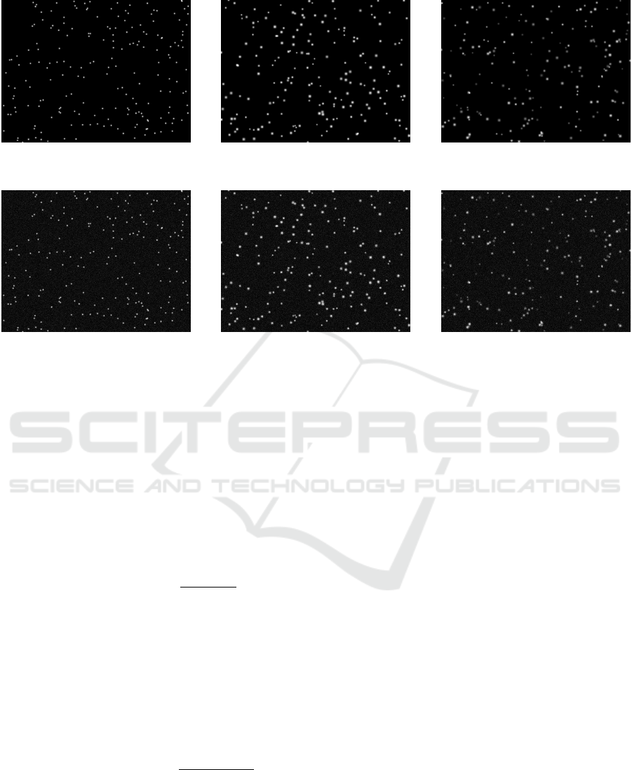
(a) Noise rate = 0%, Z

= 0% , d

10 px.

(b) Noise rate = 0%, Z

= 0 −20% ,

= 10 - 20 px.

= 10 −40% ,

= 10 - 20 px.

(d) Noise rate = 2%, Z

= 0% , d

10 px.

(e) Noise rate = 2%, Z

= 0 −20% ,

= 10 - 20 px.

(f) Noise rate = 2%, Z

= 10 −40% ,

= 10 - 20 px.

Figure 1: Samples of the synthetic dataset.

• Size and centroid positions of each particle on the

ﬁrst image are generated using a random number

generator.

• The peak intensity of each particle is based on the

Gaussian intensity proﬁle as a function of particle

depth position (Z

), efﬁciency with which the par-

ticle scatters the incident light (q) and the depth of

view (∆Z). Thus, the peak intensity of each parti-

cle I

) is (Raffel et al., 2018):

) = qexp



−

(1/8)∆Z



(1)

• Next, the intensity proﬁle across an individual

particle’s size boundary (diffusion effect) is cal-

culated by a Gaussian intensity proﬁle, which is

a function of particle peak intensity I

), par-

ticle image diameter d

−2

intensity value of

the Gaussian bell containing 95% of the scattered

light), and particle position X, Y (in pixels), given

by (Raffel et al., 2018):

I (X,Y ) = I



−

(

X−X

)

−

(

Y −Y

)

(1/8)d



(2)

• Finally, as per the ﬂow pattern, a trajectory is gen-

erated for each particle in order to have their cor-

responding positions and intensities in subsequent

image frames across a time period.

2.1.2 Dataset Properties

The following properties have been taken into con-

sideration to validate the accuracy of the system in

different scenarios which may occur in the future real

dataset.

• Size: particle size is designed as the diameter in

pixels, where some images contain ﬁxed particle

sizes while others contain a range of sizes. In

this work, we present results for a ﬁxed size of

10px, or for a range of sizes between 10px and

20px within the same image. This choice of parti-

cle size variation range is larger, on purpose than

the classical size variations of hollow glass beads

commonly used as tracers.

• Intensity: it is the intensity of the light directed

towards the particle which varies according to

Equations 1 and 2. To change the intensities, we

varied the value of the particle depth position Z

In this work, the variation of Z

is in a range of 0 -

40, i.e. corresponding to an intensity variation on

the shade of gray between 71 and 255.

• Noise: Gaussian noise has been applied to the

images. Results presented here are either for no

noise or for a variance of 2%.

• Shape: generally, all the particles are circular.

However, some of them may have a polygon

shape due to the high noise rate.

IMPROVE 2023 - 3rd International Conference on Image Processing and Vision Engineering

• Displacement: in this example, we have ﬁxed a

linear displacement of 2 pixels between 2 consec-

utive images. Other types of displacement (with

a gradient, with a rotation etc.) as well as other

displacement values have been tested, but are not

presented here.

Table 1 gathers the different parameters tested and

compared in this article, while Figure 1 shows exam-

ples of synthetic images obtained with parameters of

this table.

Table 1: Dataset properties: images of size 1024×768 px

each having 200 particles and a variation in particle inten-

sity, diameter, and noise. Particles are imposed with a linear

displacement of 2 px across subsequent image frames.

variation

(%)

(px)

Noise

variation

(%)

Images

0 %

0 10

2 10

10 to 20

0 10

2 10

0 - 20 %

0 10

2 10

10 to 20

0 10

2 10

10 - 40 %

0 10

2 10

10 to 20

0 10

2 10

2.2 Detection

The detection stage is one of the most important one

since all the upcoming stages depend on the accuracy

of detecting the particles. Figure 2 illustrates the gen-

eral diagram of the proposed detection stage. Image

binarization, ﬁlters, and non-local means denoising

algorithm have been applied to the dataset with auto-

matic conﬁguration determination considering maxi-

mizing the number of detected particles while satisfy-

ing the proposed particle diameter sizes.

2.2.1 Simple Detection Methods

After loading the images as gray-scale ones, some

well-known methodologies have been tested for de-

tecting the particles according to the predetermined

diameter sizes. For instance, image threshold bina-

rization, Difference of Gaussian (DoG), and Lapla-

cian of Gaussian (LoG).

Over the years, the basic and standard method

for individual particle detection has been the Single

Threshold Binary method. The binary method is in

Figure 2: General diagram of the detection stage.

general related to the visual properties of the parti-

cles (Ohmi and Li, 2000). Once the input image has

been pre-processed and converted into a grayscale im-

age (intensity value of each pixel is between 0 and 1),

the user can set a threshold value of intensity which

indicates to ignore all the particles having an inten-

sity above the threshold value. A Gaussian sub-pixel

location estimation method can be used to precisely

estimate the location of the center of each particle

by using a normalized auto-correlation followed by

a Gaussian ﬁtting in order to achieve sub-pixel accu-

racy. The integral coordinates of the centroid loca-

tion (X

) can be achieved from the maximum of

the auto-correlation peak (C). The exact coordinates

of each particle (X,Y) with sub-pixel accuracy can be

calculated (Raffel et al., 2018).

Difference of Gaussian (DoG) ﬁlter is a two-stage

edge detection process. In the ﬁrst step, the DoG

performs edge detection by applying a Gaussian blur

(eq. (3)) on the input image for a speciﬁed value of

standard deviation (σ

). This results in a blurred ver-

sion of the input image. This image is subtracted from

the less blurry input image resulting from the appli-

cation of another Gaussian blur with a more sharper

value of standard deviation (σ

). This difference

helps in detecting the pixel values when they cross

zero (i.e. zero crossings) i.e. when negative becomes

positive and vice versa, thus, helping in focusing on

the edges or areas of pixels having some variation

around their neighbors.

G(x,y; σ) =

√

2πσ

exp



−

+ y

2σ



(3)

The LoG is an edge detection algorithm to locate

boundaries and extract features by identifying pixel

intensity variance within the image. Generally, it is

Application of Particle Detection Methods to Solve Particle Overlapping Problems

derivative from the Gaussian ﬁlter for noise removal

by smoothing the image and Laplacian operator. The

Laplacian operator helps in highlighting the regions/

areas of rapid intensity change in the image, i.e. when

the pixel values go from negative to positive or vice

versa (i.e.zero-crossings), therefore, is a very com-

mon method used for edge detection. Equation 4,

based on Marr and Hidreth work (Marr and Hildreth,

1980) shows the mathematical representation of the

2D LoG function, centered on zero:

LoG(x,y) = −

πσ



1 −

+ y

2σ



−

2σ

(4)

It is worth mentioning that this method has been

used to detect particles within clear images. In other

words, images with no noise, and due to the presence

of different noise ratios in the rest of the images, more

advanced algorithms have been chosen to handle the

noise elimination process as explained in the next sec-

tion.

2.2.2 Non-Local Means Algorithm

With the different noise rates within the dataset, the

demand for a more efﬁcient algorithm is required to

increase image quality without affecting the edges of

the particles, hence improving the accuracy of the par-

ticle detection process.

Non-local means (NLM) is an image processing

algorithm for image denoising. it is a more advanced

technique for removing Gaussian noise from scien-

tiﬁc images that arise from electronic components

(e.g., microscope and MRI) which affects the pro-

cess of extracting information from these images. The

NLM algorithm searches the image space to calculate

the mean within non-local regions. In other words,

it is not calculating the mean based on a local group

of similar pixels (e.g., 4x4 or 9x9) as proposed by

other researchers within the same ﬁeld (Buades et al.,

2005). Instead, it is assigning the center weight CW

(the weight of the pixel to be denoised) according to

region similarity from all over the image, regardless

of their locations.

Finally, contour detection has been used to detect

the boundary of the particles and extract information

about their shape, which aims to identify the particle

center and diameter to be registered within the sys-

tem.

2.2.3 Overlapped Particles Detection

Since the particles are distributed randomly on im-

ages, this may occurring overlapping particles in

some areas. Figure 3 shows overlapped particles ex-

ample. To detect these overlapped particles, we used

template matching which is a high-level machine vi-

sion technique for determining the similarities of the

template image matrix within the source image ma-

trix (Brunelli, 2009). Prior to the use of the Template

Matching technique, we carried out two main prepro-

cessing steps. Firstly, automatically extract a good

shape template from the same source image depend-

ing on a predeﬁned particle diameter size, or by calcu-

lating all particle diameter sizes within the image and

selecting the diameter size that occurs mostly. Sec-

ondly, extracting the particles’ overlapped segments

and estimating the number of the particles depending

on the detected segment diameter and the extracted

template diameter size. The following formula shows

the process of estimating the number of overlapped

particles within the segment.

z = x ÷y (5)

No. of particles =











2 if z ≤ 2

⌈

⌋

otherwise.

(6)

where x is the diameter size of the extracted segment

and y is the diameter size of the template.

Figure 3: Overlapped particles example.

3 DETECTION RESULTS

The algorithm has been programmed in Python, a

general-purpose programming language, which has

several powerful modules in this research ﬁeld, which

will aid in the enhancement of the simplicity and scal-

ability in future research.

3.1 Detection

Several experiments and comparisons have been car-

ried out to determine the most beneﬁcial methods for

handling the process of detecting the maximum num-

ber of particles in respect of practicability, efﬁciency,

and execution time. In the ﬁrst part, we compare three

detection methods. In the second part, we improve the

results by treating the noise in the images. Finally, in

IMPROVE 2023 - 3rd International Conference on Image Processing and Vision Engineering

the third part, we reﬁne the detection thanks to an al-

gorithm allowing to minimize the problems related to

the overlapping of the particles on the same image.

3.1.1 DoG, LoG, and Binarization

As illustrated in Section 2, three techniques: DoG,

LoG, and image binarization have been taken into

consideration in the process of experimenting with the

dataset from table 1.

In addition, automatic conﬁgurations determina-

tion has been developed to ﬁnd the optimal conﬁgu-

ration in the range of 0-255 conﬁgurations that aim in

reaching the objectives. Table 2 gathers the results ob-

tained by processing the synthetic images with the 3

detection methods. We can see that the LOG method

gives the best results in the vast majority of cases.

However, the quality of the results decreases when

images are noisy. In order to minimize the noise and

to improve the detection, we used an algorithm, pre-

sented in the next section.

In addition, Figure 4 shows an example of the per-

formance comparison sample of the mentioned meth-

ods conﬁgurations on one of the test case images (Fig-

ure 4(a)) from table 2 (Z

= 10 −40, D = 10 - 20 px,

Noise = 2 %).As can be seen from Figure 4(e), Lapla-

cian of Gaussian (LoG) method was able to detect

more number of particles (N

: 176/200) as compared

to DoG method (Figure 4(b),(c)) . Although the clas-

sical Binary threshold method detects a huge number

of particles, it is clear from Figure 4(d), that in case of

a noisy image, the Binary method also detects noise as

particles. In this case, we note that another concern of

detection is related to the phenomenon of overlapping

of particles, particularly visible here when the value

of diameter detected is higher than the maximum di-

ameter generated on our synthetic images. This can

also be seen for example on Figure 5.

3.1.2 Non-Local Means Algorithm

To minimize the effect of noise on the particle detec-

tion part, non-Local Means Algorithm for gray im-

ages has been used in the proposed method with some

aiding approaches, for instance, Gaussian blur and

adaptive Gaussian thresholding, with variance algo-

rithm settings that ﬁt dataset variations in terms of the

following algorithm conﬁgurations: h-parameter de-

ciding ﬁlter strength. A higher h value leads to better

noise removal but also removes particle edges. Tem-

plate Window size and Search Window size: should

be an odd value.

Tables 3 show different settings used in the noise

removal process when the noise variance is 2%.

It is worth mentioning that the detected number

Table 2: Comparison of the detection results obtained from

the synthetic images of table 1. Results in the last three

columns Bin. DoG and LoG are given as percentages of

detected particles using respectively classical binarization,

DoG and LoG method.

(%) d

(px)

Noise

(%)

Bin.

(%)

DoG

(%)

LoG

(%)

0 67.5 95 98

2 125 77.5 96

10 to 20

0 71 91 99.5

2 97.5 90 94

0 to 20

0 70 96.5 98

2 60 96.5 93

10 to 20

0 24 88 97.5

2 60 85 96.5

10 to 40

0 64 70.5 78.5

2 87.5 77 80.5

10 to 20

0 40.5 72.5 82

2 97.5 80 88

Table 3: Parameters values and results of using NLM on 2%

Gaussian noise image.

Parameters

Setting

h 15 35 45

Template Window size 7 7 7

Search Window size 21 51 71

Result (%) 243.5 94.5 93.5

of particles represents the total number when using

the system without the overlap detection tool. Hence,

some overlapped particles are detected and counted

as a single particle. Moreover, the satisfaction of the

predetermined particle diameter sizes have been taken

into consideration as a constraint when conducting the

experiments.

Experimental results show the efﬁciency of the al-

gorithm which improves the denoising performance

and enhances image quality without affecting parti-

cle edges. Hence, increasing the detection accuracy

within the noisy dataset. Figure 6 shows the perfor-

mance of the NLM algorithm.

3.1.3 Overlap Detector Tool

Experiments have been carried out with the usage

of the overlap detector tool to maximize the de-

tected number of particles and enhance the overall

performance of the system. Open-Source Computer

Vision Library (OpenCV) provides different Single

template matching comparison methods, for in-

stance, TM SQDIFF, TM SQDIFF NORMED,

TM CCORR, TM CCORR NORMED,

Application of Particle Detection Methods to Solve Particle Overlapping Problems

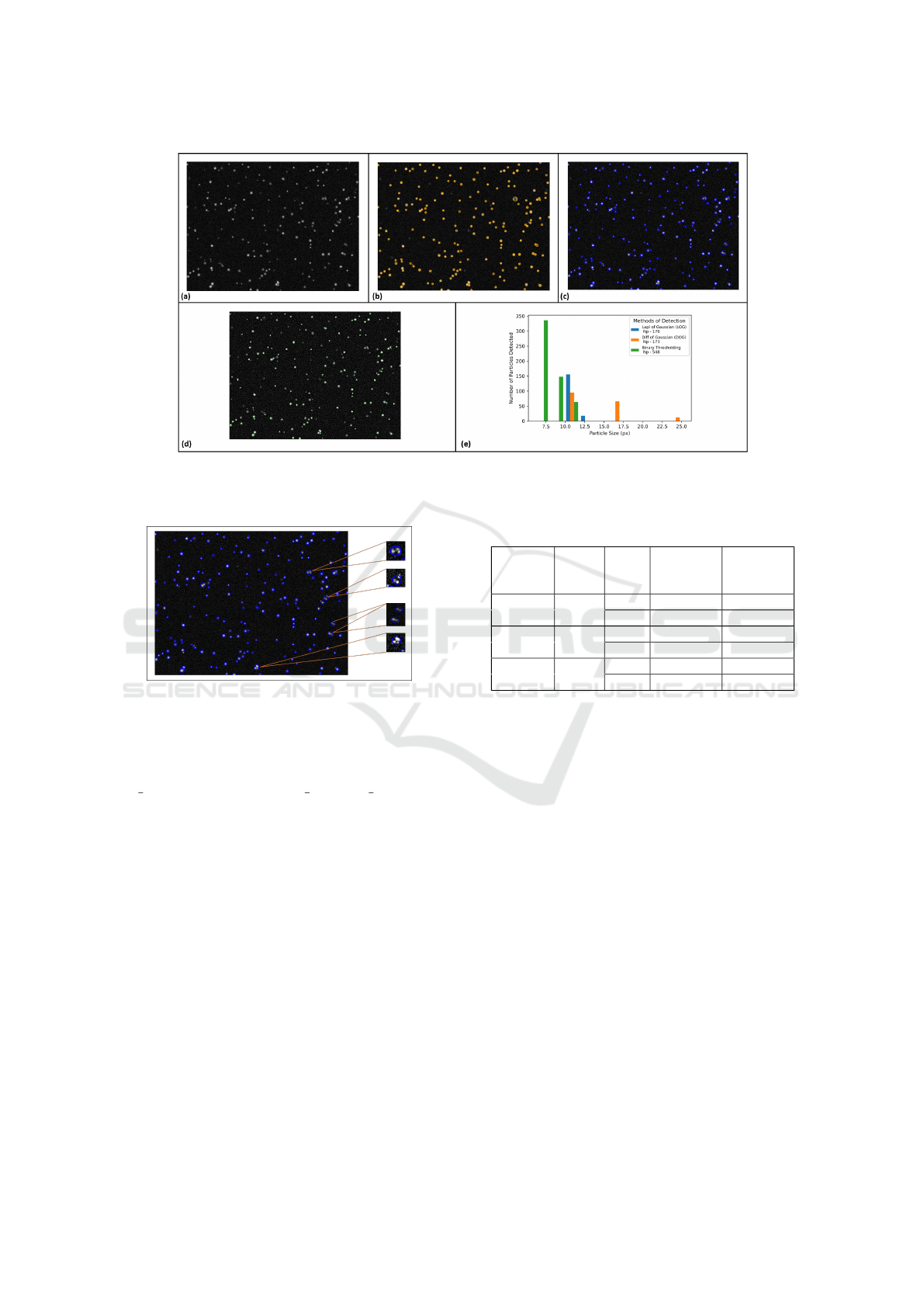
Figure 4: Performance comparison sample of DoG, LoG, and image binarization methods applied on a synthetic image with

200 particles (N), with a Diameter (d

) and variation of particle depth position ∆Z

. intensity variation of 10px ±100% and

10 −40%, respectively.

Figure 5: Occurrence of particle overlapping leading to de-

tection of particle with diameter higher than the maximum

diameter. Smaller images on the right highlights detach-

ment circles that includes one or more particles overlapped

with each other detected as one single particle.

TM CCOEFF, and TM CCOEFF NORMED.

These methods have been experimented with to

decide the most applicable method in our situation.

Additionally, the function minMaxLoc has been used

to ﬁnd the minimum and maximum result values

with their locations to extract the particles that ﬁt the

template from the overlapped region and achieve the

objectives.

Table 4 shows the number of particles detected

when using the overlap detector tool. Final experi-

ments outcomes showed highly beneﬁcial detection

rates achieved 99% within most of the datasets that

has no variation in the particle diameter size. How-

ever, some of the overlapped particles could not be

detected because of their coordinates lying on the bor-

ders within the images. Figure 7 shows a result exam-

ple of using the overlap detector tool and statistics.

Table 4: The result of using overlap detector tool.

∆Z

(%)

(px)

Noise

(%)

Without

Overlap

tool (%)

With

Overlap

tool (%)

0 10

0 89 99

2 85 95

0 to 20 10

0 93 99

2 92.5 98.5

10 to 40 10

0 87 99.5

2 76 91

4 CONCLUSIONS

There can be no doubt that detecting the microscopic

featureless particles in liquids with various proper-

ties is challenging. Although different research con-

texts in this ﬁeld, it was found that using Laplacian

of Gaussian and non-local means algorithms with au-

tomatic conﬁguration determination is highly beneﬁ-

cial in the detection stage and aims the precise de-

termination of the particle center and diameter. Fur-

thermore, the overlap detector tool enhanced the out-

comes and showed a highly beneﬁcial estimation rate

yields maximizing the detected number of particles

for the current research synthetic dataset. However,

further research must be conducted to enhance the de-

tection rates of different noise ratio datasets, includ-

ing the usage of a multi-template matching technique

to handle the analysis process of different particle di-

ameter sizes within the same image.

IMPROVE 2023 - 3rd International Conference on Image Processing and Vision Engineering

(a) Noise rate= 0%. (b) Noise rate= 2%. (c) NLM algorithm performance.

Figure 6: The performance of the NLM algorithm.

(a) When using overlap detector tool:

detection accuracy of 99%.

(b) Without using overlap detector

tool : detection accuracy of 89%.

detector tool.

Figure 7: The performance of the overlap detector tool.

REFERENCES

Baek, S. J. and Lee, S. J. (1996). A new two-frame particle

tracking algorithm using match probability. Experi-

ments in Fluids, 22(1):23–32.

Brunelli, R. (2009). Template matching techniques in com-

puter vision: theory and practice. John Wiley & Sons.

Buades, A., Coll, B., and Morel, J.-M. (2005). A non-local

algorithm for image denoising. In 2005 IEEE Com-

puter Society Conference on Computer Vision and

Pattern Recognition (CVPR’05), volume 2, pages 60–

65 vol. 2.

Heyman, J. (2019). TracTrac: A fast multi-object tracking

algorithm for motion estimation. Computers & Geo-

sciences, 128:11–18.

Janke, T., Schwarze, R., and Bauer, K. (2020). Part2track:

A matlab package for double frame and time resolved

particle tracking velocimetry. SoftwareX, 11:100413.

Katiyar, S. K. and Arun, P. V. (2014). Comparative analysis

of common edge detection techniques in context of

object extraction.

Kim, H.-B. and Lee, S.-J. (2002). Performance improve-

ment of two-frame particle tracking velocimetry using

a hybrid adaptive scheme. Measurement Science and

Technology, 13(4):573–582.

Lee, S., Yoon, G., and Go, T. (2019). Deep learning-based

accurate and rapid tracking of 3d positional informa-

tion of microparticles using digital holographic mi-

croscopy. Experiments in Fluids, 60.

Lefta, A. S., Daway, H. G., and Jouda, J. (2022). Red

blood cells detecting depending on binary conversion

at multi threshold values. Al-Mustansiriyah Journal

of Science, 33(1):69–76.

Lima, R., Ishikawa, T., Imai, Y., and Yamaguchi, T. (2012).

Confocal micro-piv/ptv measurements of the blood

ﬂow in micro-channels. Micro and Nano Flow Sys-

tems for Bioanalysis, page 131–151.

Marr, D. and Hildreth, E. (1980). Theory of edge detection.

The Royal Society of London. Series B. Biological Sci-

ences, 207(1167):187–217.

Mohr, D. P., Knapek, C. A., Huber, P., and Zaehringer, E.

(2019). Algorithms for particle detection in complex

plasmas. Journal of Imaging, 5(2).

Ohmi, K. and Li, H.-Y. (2000). Particle-tracking velocime-

try with new algorithms. Measurement Science and

Technology, 11(6):603–616.

Qian, Y., Ji, R., Duan, Y., and Yang, R. (2021). Multiple

object tracking for occluded particles. IEEE Access,

9:1524–1532.

Raffel, M., Willert, C., Scarano, F., K

ahler, C., Wereley, S.,

and Kompenhans, J. (2018). Particle Image Velocime-

try A Practical Guide. Springer.

Scharnowski, S. and K

ahler, C. J. (2020). Particle im-

age velocimetry - classical operating rules from to-

day’s perspective. Optics and Lasers in Engineering,

135:106185.

Thielicke, W. (2021). Digital particle image velocimetry

tool for matlab.

Application of Particle Detection Methods to Solve Particle Overlapping Problems