Forecasting Residential Energy Consumption: A Case Study for Greece

Dimitra Kouvara

and Dimitrios Vogiatzis

The American College of Greece, Deree Athens, Greece

The American College of Greece, Deree & NCSR “Demokritos” Athens, Greece

Keywords:

Industrial Applications of Artiﬁcial Intelligence, Energy Consumption Forecasting, Time-Series Forecasting.

Abstract:

Residential energy consumption forecasting has immense value in energy efﬁciency and sustainability. In

the current work we tried to forecast energy consumption on residences in Athens, Greece. As a proof of

concept, smart sensors were installed into two residences that recorded energy consumption, as well as indoors

environmental variables (humidity and temperature). It should be noted that the data set was collected during

the COVID-19 pandemic. Moreover, we integrated weather data from a public weather site. A dashboard was

designed to facilitate monitoring of the sensors’ data. We addressed various issues related to data quality and

then we tried different models to forecast daily energy consumption. In particular, LSTM neural networks,

ARIMA, SARIMA, SARIMAX and Facebook (FB) Prophet were tested. Overall SARIMA and FB Prophet

had the best performance.

1 INTRODUCTION

Electricity was invented in 1752. Over the years and

as technology advanced, electricity evolved from be-

ing a commodity mostly enjoyed by the upper class

to a service available in every household. But as

the population grows and production is heading to a

green model, meanwhile energy prices are increasing,

which makes someone wonder if having electricity in

the future will be once again considered a luxury (Seel

et al., 2018). Since the beginning of 2022 and es-

pecially since the recent turmoil in Eastern Europe,

a rally of increasing prices in energy was registered

globally with many European countries being more

vulnerable to the current energy crisis. It is easily un-

derstood that the energy crisis is not a temporary state

but a problem that the whole world needs to address

and ﬁnd innovative ideas to confront it.

To resolve the energy crisis in Europe, many Eu-

ropean countries such as Spain, Italy, Greece and UK,

adopted national measures to avert the crisis, such as

offering subsidies to energy providers and imposing

price caps, in order to shield citizens from rising elec-

tricity costs as their economies recover fully from the

COVID-19 pandemic (Ozili and Ozen, 2021). On the

other hand, consumers are interesting in ways that

help them reduce their energy consumption without

compromising their needs. A technological advance-

ment that contributed to this issue is the ability to

turn most of the devices that people use daily into

smart ones (Tom et al., 2019). With the rise of 4G

and more recently 5G, these smart devices are able

to connect to the internet and be utilized by the user

remotely. Nowadays, bulbs can turn off when a per-

son leaves the room, thermostats can adjust to energy

needs on the ﬂy, other appliances can notify the user

of energy leaks and much more. The idea that led

to this is the Internet of Things (IoT), a network of

physical objects that use sensors, software and other

technologies to connect to each other and exchange

data between them over the internet. Grids and Smart

Homes, along with signiﬁcant Information and Com-

munication Technology developments, will leverage

the future energy system paradigm, where digitally

based marketplaces will allow consumers to easily

trade energy and services (Soto et al., 2021).

Contribution

In the current work the goal was to forecast energy

demand at the level of individual residence. To this

end, we installed smart sensors in over 20 different

residences to gather energy and (indoor) weather re-

lated readings. We also dealt with the quality of the

data coming form the sensors. We evaluated machine

learning models for time-series to predict the daily

energy consumption over a period of one week. In

particular we applied ARIMA models, FB Prophet

and LSTM Neural Networks. Furthermore, a dash-

484

Kouvara, D. and Vogiatzis, D.

Forecasting Residential Energy Consumption: A Case Study for Greece.

DOI: 10.5220/0011854500003467

In Proceedings of the 25th International Conference on Enterprise Information Systems (ICEIS 2023) - Volume 1, pages 484-492

ISBN: 978-989-758-648-4; ISSN: 2184-4992

 2023 by SCITEPRESS – Science and Technology Publications, Lda. Under CC license (CC BY-NC-ND 4.0)

board was developed for visualizing historical and

forecasted data. The dashboard can be accessed by

the end customer, or remotely by the electric com-

pany.

The rest of the paper is organized as follows. In

Section 2 we refer to previous work on energy pre-

diction. Then in Section 3 we refer to the forecasting

models and also to the dashboard that was designed.

Following, Section 4 refers to data harvesting, and

data quality issues. Forecasting results are presented

in Section 5. Finally, conclusions are drawn in Sec-

tion 6.

2 RELATED WORK

There have been many efforts to predict energy de-

mand, but the prediction task differs depending on the

time horizon, e.g. long-term, medium-term or short-

term; the focus on the prediction, for instance av-

erage energy demand over peak energy demand and

whether features beyond past samples of energy de-

mand are used. Moreover, pre-processing of the data

as well as handling data quality issues is important.

For instance in (Chaturvedi et al., 2022), the au-

thors compared various time-series models to pre-

dict total monthly and peak monthly demand in In-

dia. In particular SARIMA, LSTM RNN and FB

Prophet have been evaluated. FB Prophet along with

SARIMA have been the most accurate with LSTM

being exhibiting lower performance.

Predicting building energy consumption is an-

other area that has been investigated (Bourdeau et al.,

2019), (Amasyali and El-Gohary, 2018). Various

models have been considered including Autoregres-

sive Models (AR), Artiﬁcial Neural Networks (ANN)

and Ensemble methods. Also unsupervised tech-

niques, reinforcement learning (RL) and transfer

learning have been tried.

The evaluation results are not directly comparable,

as they were applied on different not publicly avail-

able data sets. However, there has been a recent inter-

national competition on a publicly available data set

to predict energy consumption on buildings (Miller

et al., 2022). This may be a good starting point for

the comparison of different models.

3 METHODOLOGY

In this section, the pipeline of the time-series predic-

tion along with a detailed reference to the applied ma-

https://www.kaggle.com/c/ashrae-energy-prediction

chine learning models is being presented. (See also

Figure 2).

3.1 Pipeline of Time-Series Prediction

We address the problem of forecasting the daily en-

ergy consumption of residences over a period of

one week. We used models based on econometrics:

auto-regressive integrated moving average (ARIMA)

and its successors, seasonal ARIMA (SARIMA) and

SARIMA with exogenous factors (SARIMAX). We

also used the FB Prophet and the Long Short-Term

Memory (LSTM) Neural Network. The three models

were trained using data from 2019 to 2022, and they

were evaluated on data from 2022. The evaluation

metrics employed were the root mean squared error

(RMSE), mean absolute error (MAE), mean absolute

percentage error (MAPE) and the R-squared (R

). Fi-

nally, there was developed a dashboard to visualize

energy and indoor environmental data.

ARIMA Models

ARIMA models are widely used econometric ap-

proaches to uni-variate time-series modeling (Box

et al., 2015), (Shumway et al., 2000). It is actually

a class of models that explain a time-series based on

its own past values. In particular, it uses its own lags

and the lagged forecast errors, so as to predict future

values. All three above-mentioned ARIMA variations

(ARIMA, SARIMA and SARIMAX)

are considered

to be tools for time-series forecasting. The difference

between ARIMA and SARIMAX is the seasonality

and exogenous factors. ARIMA model is character-

ized by three parameters: p is the order of the AR

term, q is the order of the MA term and d is the num-

ber of differencing required to make the time-series

stationary. SARIMAX requires an extra set of p,

d, and q parameters for the seasonality aspect, and

an s parameter that is the periodicity seasonal cycle

of the data. The parameters of the ARIMA models

are usually determined by the auto-correlation func-

tion (ACF) and by the partial auto-correlation func-

tion (PACF).

Facebook Prophet

Prophet is an open-source tool developed by Face-

book in 2017 for the prediction of time-series val-

ues (Taylor and Letham, 2018). It has been used in

different business applications and is available both in

https://github.com/statsmodels/statsmodels/tree/main/

statsmodels/tsa

Forecasting Residential Energy Consumption: A Case Study for Greece

485

Python and R.

It is an additive model featuring a de-

composed time-series with three components: trend

g(t), seasonality s(t), holidays h(t) (optional term)

and an error term (ε

) that stands for random ﬂuc-

tuations that cannot be explained by the model, and

which are assumed to be normally distributed.

LSTM Recurrent Neural Network Model

The LSTM Recurrent Neural Network model was

proposed in 1997 and it is widely used in forecast-

ing (Hochreiter and Schmidhuber, 1997), (Greff et al.,

2016). LSMTs are complex models, i.e. in general

they need much more effort to optimize them. Many

parameters, such as the number of layers, epochs,

batch size, activation functions, optimizer, have to be

properly tuned, in order to get the best possible re-

sults. We have used the Keras library

Dashboard

A dashboard named Home Assistant Administrator’s

Interface was designed with Microsoft Power BI.

The purpose of the dashboard is to allow users to

monitor the sensors installed in residences (see Fig-

ure 1). The dashboard consists of a homepage, con-

taining the logo of the telecommunications company

along with the report’s name, and an interactive rib-

bon on the left part of the page with buttons that allow

the user to navigate through several pages.

There are pages dedicated to the residential en-

ergy consumption analysis, that display statistical

data (e.g. minimum and maximum energy readings).

Also it provides energy readings for speciﬁc years,

months, weeks, or days including the number of de-

tected sensors’ malfunctions. A donut shaped chart,

a tree-map, and a column chart are constructed, each

one depicting the average energy consumption of the

residence based on the years, months, and days re-

spectively. The color palette allows the user to inspect

and detect the periods of high energy consumption

and draw meaningful insights. Lastly, a Prediction

Analysis page is available, where the user can view

the daily predictions of the energy consumption over a

week for each model developed on the project, as well

as the actual energy readings. There is an additional

card containing the evaluation metrics (MAPE, MSE,

RMSE and R

) of each prediction model and another

one for the execution time in seconds. A gauge visual

depicts the average of the residuals of each model,

along with the minimum and maximum values and

https://github.com/facebook/prophet

https://www.tensorﬂow.org/api docs/python/tf/keras/

layers/LSTM

https://powerbi.microsoft.com/en-au/

another card shows the percentage of days that were

predicted over the whole spectrum of days contained

in the data set. The column chart is utilized for the

comparison of the actual and predicted consumption

values per day and uses a line to show their residuals.

All report’s pages are interactive and contain ar-

row and navigation buttons to move to the next page

and to a chosen analysis tab, respectively.

Figure 1: A user dashboard to monitor residential sensors.

4 DATA SET HARVESTING

We retrieved data from the smart sensors installed

in two residences, to train models for energy con-

sumption forecasting. A Non-Disclosure Agreement

(NDA) was signed between the OTE Academy,

a subsidiary of OTE, which is one of the largest

telecommunication companies in Greece, and the au-

thors. Since the smart sensors collected personal in-

formation of the customers, it was ensured that the

whole process would comply with the General Data

Protection Regulation (GDPR).

The NDA required

to handle all data with strict conﬁdentiality, and take

all the appropriate measures so the data is stored

safely and used only for the purpose of the current

work.

Environmental sensors have been installed in the

two residences that measure indoor humidity and in-

door temperature. Moreover there are power meters

installed at the residences’ switchboards which record

power and energy consumption. All the data were

harvested and subsequently stored in InﬂuxDB,

time-series highly optimized database. The data were

retrieved from InﬂuxDB in a JSON format to facil-

itate post-processing and interoperability with other

system components.

The data set was enriched with weather data, and

in particular with the outdoor temperature and out-

https://oteacademy.gr/en/

https://www.gdpreu.org/

https://www.inﬂuxdata.com/

ICEIS 2023 - 25th International Conference on Enterprise Information Systems

486

Figure 2: The pipeline of the energy consumption predic-

tion.

door humidity. These data were collected through a

free API from the World Weather Online.

4.1 Data Description

As a proof of concept, we used data from two differ-

ent residences, both of which are situated in Athens,

Greece. The installation of the ﬁrst sensors to the

residences started in June 2019, and data were col-

lected from that time and for a period of two years.

We have also collected weather related data for the

same period. Both the sensor and weather data refer

to hourly data points. Some descriptive statistics of

the acquired sensor and weather related data sets are

depicted in Table 1.

Table 1: Statistics of the data sets (2019–2022).

Residence 1

cumulative

energy

[kWh]

power [W] temperature

[

◦

humidity

[%]

mean 2296.50 19881.96 21.14 62.44

std 1554.35 60317.96 4.13 8.75

min 5.39 -40980.86 13.03 32.07

max 27083.62 3623000 31.83 85.73

missing values 5.53% 5.53% 3.85% 3.85%

#samples 24,239 24,239 19,904 19,904

Residence 2

cumulative

energy

[kWh]

power [W] temperature

[

◦

humidity

[%]

mean 7350.65 2388.58 20.85 67.49

std 2043.66 7790.89 4.06 12.18

min 3498.92 0 13.25 30.33

max 13861.59 140739.83 30.90 99.52

missing values 3.21% 3.58% 4.07% 4.07%

#samples 23,852 23,760 14,003 14,003

4.2 Data Quality

Poor-quality data is often pegged as the source

of operational snafus, inaccurate analytics, and ill-

conceived business strategies (Batini et al., 2016). Be-

sides, the main challenge of this study was the data

pre-processing phase, since data in the real world

is often dirty and corrupted with inconsistencies,

noise, incomplete information, and missing values,

and therefore data quality should be recognized and

addressed.

https://www.worldweatheronline.com/

The ﬁrst step was the exploration of the raw data to

detect any sensor malfunction before performing pre-

processing. Both energy and weather data collected

by the power meters and the environmental sensors

were examined in terms of data quality, as any de-

tected inconsistencies directly affect the performance

of the predictive models.

Energy Related Sensor Malfunctions

Erroneous readings from the power meters were re-

lated to many causes. First, internet connection dis-

ruptions, and power failures resulted in missing val-

ues. Second, hardware problems caused lags. This

resulted in energy values that were constant for ex-

tended periods of time or even resulted in energy

spikes, which is unusual (see Figure 3).

Figure 3: Cumulative energy through time: At about 16,000

hours the curve drops from about 12,000kWh to about

6,000kWh. A clear case of sensor malfunction.

Environment Related Sensor Malfunctions

A rough way to check for sensor lags is by visually in-

specting the time-series. For instance, Figures 4 and 5

depict temperature and humidity over time. Miss-

ing values occurred at about 12,000 hours (about 1.5

years from the beginning of the time series). Also,

some very prominent spikes are indicative of some

malfunction.

4.3 Feature Extraction

The extraction of temporal features was proven criti-

cal in analyzing the energy consumption of the resi-

dences. The exact hour, day, month and year as well

as the time intervals that correspond to working hours,

or to busy hours were essential pieces of informa-

tion. We used the Python holidays library

to iden-

https://python-holidays.readthedocs.io/en/latest/#

Forecasting Residential Energy Consumption: A Case Study for Greece

487

Figure 4: Indoor temperature, missing values around

12,000h.

Figure 5: Indoor humidity, missing values around 12,000h.

tify Greek holidays, a factor that could likely affect

the energy consumption, as on public holidays people

behave differently. Moreover, features related to the

sunrise, sunset time, and daylight duration were ex-

tracted from information included in the weather data.

Finally, since the sensors reported cumulative en-

ergy, we had to subtract two neighboring values to

obtain the energy consumption per hour. The training

data set comprised hourly measurements. The fore-

casting was performed on a daily basis for up to 7

days (see Table 2 for an overview of the data features).

4.4 Data Cleaning

Sensor malfunctions affected to a great extend the

data quality. In particular we detected and addressed

the following types of data quality issues: missing

values, outliers and other suspicious data.

First, we applied a z-score value of 4 to remove

cumulative energy, indoor temperature and indoor

humidity outliers. Then, we replaced the missing en-

vironmental values with their adjacent values by uti-

lizing the forward ﬁll function of Pandas in Python;

this propagates the last valid observation forward

Following that, we dealt with the suspicious en-

ergy values that are due to hardware problems, includ-

ing internet connection disruptions and power fail-

ures. This caused missing values. Sensor malfunc-

tions caused lags that occurred for extended periods

of time. This was observed as constant energy values

or as energy spikes.

As far as the malfunctions due to internet connec-

tion issues were concerned, we replaced the missing

energy values by the mean and smoothing the line

between those two points, since we had two correct

points of reference. That was possible due to the fact

that after the internet connection was restored, the

sensor’s measurements would revert to the correct en-

ergy values.

Addressing the energy spikes and the constant en-

ergy values was more challenging. First, we per-

formed time-series data visualization with Grafana.

We observed that the sensors were lagging for ex-

tended time periods, as they were returning the same

energy value for the many consecutive time steps.

• For the energy per hour feature (see also Sec-

tion 4.3), the z-score outlier detection method was

applied again to remove any abnormally high en-

ergy values. These values were then replaced with

their adjacent energy values by using the forward

ﬁll function of Pandas. Such values were ob-

served in a few occasions, something that could

be the result of a sensor’s malfunction or an ex-

treme but still actual event.

• The detection of the constant energy values was

based on domain experts’ advice that the mini-

mum energy consumed at each data point should

be more that 0.06kWh. Thus in the case that we

detected a series of 3 or more consecutive data

points in the time-series where the energy con-

sumption was below that threshold, the values

were replaced with the mean value of their ad-

jacent ones. Constant energy values lasting for a

whole month values were observed in residence 2.

It was an extreme case of corrupt values in terms

of duration.

5 FORECASTING RESULTS

In this section we report the forecasting experiments

with ARIMA, SARIMA, SARIMAX, FB Prophet and

https://pandas.pydata.org/docs/reference/api/pandas.

DataFrame.fﬁll.html

https://grafana.com/

ICEIS 2023 - 25th International Conference on Enterprise Information Systems

488

Table 2: Extracted features of the time-series data.

Feature Name Format

Time-based features

Year timestamp (form: 2019)

Month timestamp (form: Jan 1 - Dec 12)

Date timestamp (form: 2019-06-27)

Day timestamp (form: 27)

Day of week timestamp (form: Mon 0 - Sun 6)

Time timestamp (form: 09:00:00)

Hour timestamp (form: 9)

Weekday 1 if day of week < 5, else 0

Working Hours 1 if hour in range [9:00, 18:00] & day of week

<= 5, else 0

Busy hours 1 if hour in range [7:00, 9:00] or [19:00, 00:30]

in weekdays or hour in range [9:00, 15:00] in

weekends

Holiday NoHoliday, MondayoftheHolySpirit, Easter-

Monday, IndependenceDay, DayafterChrist-

mas, Labourday, OchiDay, Epiphany, Clean-

Monday, AssumptionofMary, NewYearsDay,

Christmas

Weather-based features

Sunrise conversion to strptime() (form: 1561601100.0)

Sunset conversion to strptime() (form: 1561654320.0)

Is day light 1 if sunrise ≤ time ≤ sunset, else 0

Sensor-based features

Energy per hour energy value (form 0.0)

LSTM models, along with their evaluation.

In ARIMA, SARIMA and FB Prophet, the en-

ergy, date and year features of the data were selected.

In SARIMAX the environmental parameters indoor

temperature and humidity were included as the ex-

ogenous variables. Finally, in the LSTM the energy,

indoor and outdoor environmental parameters along

with the features listed in Table 2 were selected.

ARIMA Results

First we considered ARIMA models, to provide a

baseline performance benchmark with which to com-

pare the rest of the models. Overall it has a poor

performance. This was due to the fact that although

ARIMA can handle data with an underlying trend, it

fails to support time-series with a seasonal compo-

nent. The model’s performance is depicted in Fig-

ures 6 and 7 for residences 1 and 2 respectively.

Figure 6: ARIMA Forecast for Residence 1.

In an attempt to improve the prediction, ARIMA’s

successors SARIMA and SARIMAX were applied.

A grid search discovered the best parameters for

the model with the augmented Dickey-Fuller (ADF)

and Akaike Information Criterion (AIC) metrics.

Figure 7: ARIMA Forecast for Residence 2.

The best results were for (p, d, q) = (0, 1, 0) and

for (P, D, Q, M) = (1,1, 1, 7), where the (p, d, q) and

(P, D, Q, M) terms refer to the order of the time-series

and the order of the seasonal component respectively.

The experiments have shown that SARIMA with

only the energy feature, resulted in slightly better pre-

dictions compared to SARIMAX, that included the

indoor temperature and humidity values (See Fig-

ures 8 and 9 for the results).

Figure 8: SARIMA Forecast Line Plot for Residence 1.

Figure 9: SARIMA Forecast Line Plot for Residence 2.

Facebook Prophet Results

In FB Prophet the trend changepoints prior scale (τ)

and seasonality prior scale (σ) hyper-parameters can

be tuned so that the model ﬁts data optimally. After

experimentation, the daily, weekly, and yearly sea-

sonality parameters of the model were set to true,

whereas the period indicating the number of the prior

periods that are important for the prediction was set

to 1. The last parameter that we considered was the

Fourier order, which is responsible for estimating the

Forecasting Residential Energy Consumption: A Case Study for Greece

489

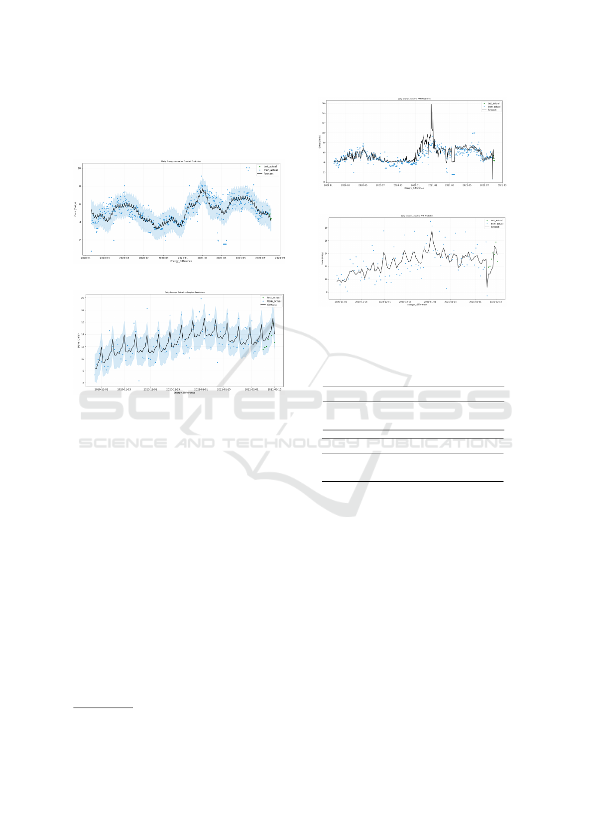
seasonality and whose value was set to 8.

After selecting the best values of the parameters,

we employed them to evaluate the FB Prophet model

in the test phase. The results for the two residences

are presented in Figures 10 and 11 respectively.

Figure 10: FB Prophet forecasting for residence 1.

Figure 11: FB Prophet forecast for residence 2.

The FB Prophet offers additional features as exter-

nal sources, such as custom holidays, vacation days,

and even a custom seasonality that could be based on

the user’s behavior. However, since the predictions

were pretty accurate, the exploration of these features

was left for future work.

LSTM Recurrent Neural Network Results

The architecture of the LSTM in Keras

consists of

an LSTM layer, dense and dropout layers for pre-

vention against over-ﬁtting. The Adam optimizer

was used, and the optimization was based on mean

squared error (MSE). Finally, the model was trained

for 10 epochs with a batch size of 64. The forecasting

lines of the LSTM model for both residences can be

observed in Figures 12 and 13.

Comparison of Models

We rated the performance of the models on the time-

series data based on the MSE, MAPE, RMSE (lower

values are better) and R

(higher values are better)

metrics. The results for both the training and test-

ing phases, along with the models’ execution time are

https://keras.io/

Figure 12: LSTM Forecast Line Plot for Residence 1.

Figure 13: LSTM Forecast Line Plot for Residence 2.

presented for both of the residences in Tables 3 and 4.

Table 3: Evaluation metrics for residence 1.

Training set residence 1

Models MSE MAPE RMSE R

Execution

time [sec]

ARIMA 0.76 0.87 11.26 0.62 47

SARIMA 0.78 0.88 12.05 0.61 47

Prophet 0.93 0.96 16.96 0.53 48

LSTM 1.32 1.15 16.48 0.35 59

Testing set residence 1

Models MSE MAPE RMSE R

Execution

time [sec]

ARIMA 0.14 0.37 6.37 -0.27 47

SARIMA 0.29 0.55 10.49 -1.72 47

Prophet 0.11 0.33 5.75 0.02 48

LSTM 0.78 0.88 15.98 -5.55 59

6 CONCLUSIONS

In the current work we tried to forecast the energy

consumption in two residences. We used data col-

lected from sensors in the residences (energy con-

sumption and environmental data) as well as weather

data (outdoor data). We dealt with data quality issues

stemming from the operation of the sensors and the

internet connection.

Different models were tested for forecasting the

energy consumption. The best models were as ex-

pected the SARIMA and FB Prophet that had a good

accuracy. As far as the LSTM’s performance is con-

cerned, there was evidence that further optimization

of its parameters would improve its results.

Overall the models that used only the energy con-

sumption feature to make predictions had a better

performance. This was probably caused because the

ICEIS 2023 - 25th International Conference on Enterprise Information Systems

490

Table 4: Evaluation metrics for residence 2.

Training set residence 2

Models MSE MAPE RMSE R

Execution

time [sec]

ARIMA 8.20 2.86 18.32 -0.37 24

SARIMA 8.23 2.87 18.81 -0.37 24

Prophet 3.18 1.78 11.23 0.47 24

LSTM 2.67 1.63 11.11 0.53 29

Testing set residence 2

Models MSE MAPE RMSE R

Execution

time [sec]

ARIMA 6.90 2.63 19.02 -2.92 24

SARIMA 0.41 0.64 4.16 0.77 24

Prophet 1.09 1.05 7.19 0.38 24

LSTM 1.96 1.40 9.95 -0.26 29

available data set was not large enough. Also the data

were collected during the COVID-19 pandemic, when

the subsequent lockdown periods caused an unusual

behavior on the part of the consumers. The data were

collected over the past three years, but each year was

different. In 2019 the residents’ behavior was nor-

mal, since there was no lockdown, but in 2020 all

changed since people had to stay at home and thus the

energy consumption increased (Abu-Rayash and Din-

cer, 2020). Abnormalities like these heavily affect the

data especially in the seasonality aspect, that is crucial

for time-series data as the ones in hand. This might be

the reason of models performing worse when no ex-

ternal data are utilized, since the target variable that is

used is compromised. Moreover, all the models, ex-

cept FB Prophet performed worse with large sizes of

training data. The FB Prophet had better performance

with a larger size of training data.

Concluding, the forecasting models are part of a

software service that is accessible via a dashboard.

The service can be used by the customer to moni-

tor historical energy consumption, obtain predictions

and thus to draw conclusions providing a better under-

standing of the residence’s energy consumption, and

to possibly take actions in economizing. The service

can also be used by the electric company to acquire

sensor data from all residences. The company could

possibly “intervene” in the residence by switching off

unused smart plugs should they have the customer’s

consent; or even to suggest ways to reduce the resi-

dential energy consumption by replacing old and in-

efﬁcient domestic appliances, i.e., oven, fridge, wash-

ing machine.

The current work can be expanded in several di-

rections. First, we can try to predict energy consump-

tion based on all 20 residences instead of only 2. Sec-

ond, as data continue to be gathered we could enhance

the training data sets. Finally, we could try different

forecasting models such as the transformer networks.

ACKNOWLEDGEMENTS

We would like to thank OTE Academy for provid-

ing the data, and the American College of Greece,

Deree for supporting the current work, as well as

Mr. Theodoros Diamantopoulos and Mr. Dimitrios

Salmatanis for their contribution to this project.

REFERENCES

Abu-Rayash, A. and Dincer, I. (2020). Analysis of the

electricity demand trends amidst the covid-19 coron-

avirus pandemic. Energy Research & Social Science,

68:101682.

Amasyali, K. and El-Gohary, N. M. (2018). A review of

data-driven building energy consumption prediction

studies. Renewable and Sustainable Energy Reviews,

81:1192–1205.

Batini, C., Scannapieco, M., et al. (2016). Data and infor-

mation quality. Cham, Switzerland: Springer Interna-

tional Publishing.

Bourdeau, M., qiang Zhai, X., Nefzaoui, E., Guo, X.,

and Chatellier, P. (2019). Modeling and forecast-

ing building energy consumption: A review of data-

driven techniques. Sustainable Cities and Society,

48:101533.

Box, G. E., Jenkins, G. M., Reinsel, G. C., and Ljung, G. M.

(2015). Time series analysis: forecasting and control.

John Wiley & Sons.

Chaturvedi, S., Rajasekar, E., Natarajan, S., and McCullen,

N. (2022). A comparative assessment of sarima, lstm

rnn and fb prophet models to forecast total and peak

monthly energy demand for india. Energy Policy,

168:113097.

Greff, K., Srivastava, R. K., Koutn

ık, J., Steunebrink, B. R.,

and Schmidhuber, J. (2016). Lstm: A search space

odyssey. IEEE transactions on neural networks and

learning systems, 28(10):2222–2232.

Hochreiter, S. and Schmidhuber, J. (1997). Long short-term

memory. Neural computation, 9(8):1735–1780.

Miller, C., Picchetti, B., Fu, C., and Pantelic, J. (2022).

Limitations of machine learning for building energy

prediction: Ashrae great energy predictor iii kaggle

competition error analysis. Science and Technology

for the Built Environment, pages 1–18.

Ozili, P. K. and Ozen, E. (2021). Global energy crisis: im-

pact on the global economy. In Proceedings of IAC in

Budapest 2021, volume 1, pages 85–89. Czech Insti-

tute of Academic Education.

Seel, J., Mills, A. D., and Wiser, R. H. (2018). Impacts of

high variable renewable energy futures on wholesale

electricity prices, and on electric-sector decision mak-

ing. Lawrence Berkeley National Laboratory (May

2018).

Shumway, R. H., Stoffer, D. S., and Stoffer, D. S. (2000).

Time series analysis and its applications, volume 3.

Springer.

Forecasting Residential Energy Consumption: A Case Study for Greece

491

Soto, E. A., Bosman, L. B., Wollega, E., and Leon-Salas,

W. D. (2021). Peer-to-peer energy trading: A review

of the literature. Applied Energy, 283:116268.

Taylor, S. J. and Letham, B. (2018). Forecasting at scale.

The American Statistician, 72(1):37–45.

Tom, R. J., Sankaranarayanan, S., and Rodrigues, J. J. P. C.

(2019). Smart energy management and demand re-

duction by consumers and utilities in an iot-fog-based

power distribution system. IEEE Internet of Things

Journal, 6(5):7386–7394.

ICEIS 2023 - 25th International Conference on Enterprise Information Systems

492