On-the-Fly Acquisition and Rendering with Low Cost LiDAR and RGB
Cameras for Marine Navigation
Somnath Dutta
a
, Fabio Ganovelli
b
and Paolo Cignoni
c
Institute of Information Science and Technologies “Alessandro Faedo” (ISTI), Italian National Research Council (CNR),
Via Giuseppe Moruzzi 1, 56124 Pisa, Italy
Keywords:
LiDAR-RGB Images Calibration, Computer Graphics.
Abstract:
This paper describes a hardware/software system, dubbed NausicaaVR, for acquiring and rendering 3D envi-
ronments in the context of marine navigation. Like other similar work, it focuses on system calibration and
rendering but the specific context poses new and more difficult challenges for the development when com-
pared to the classic automotive scenario. We provide a comprehensive description of all the components of
the system, explicitly reporting on encountered problems and subtle choices to overcome those, in an attempt
to render an insightful picture of how this and similar systems are built.
1 INTRODUCTION
The proliferation of high-quality depth sensors and
cameras at an affordable price has enriched the do-
main of graphics and vision and consequently resulted
in the development of advanced applications cover-
ing broad disciplines. Among those applications,
there is a certain proportion that intends to present in-
formation to the user in an elementary fashion and
specifically related to the situation and environment.
Cameras have been the predominant choice for a vi-
sual navigational system, however, with the increas-
ing availability of depth sensors, the geometric un-
derstandings added an extra dimension to the entire
visual navigational ecosystem.
Marine navigation, often subjected to adverse weather
and lighting conditions, has traditionally relied on the
intensive manual labor of its crew. Alike land or
aerial navigational systems, cameras are the prefer-
able choice and are now augmented with 3D sensors,
for instance, Lidars. Traditionally, marine vessels, for
instance, ships and boats, relied on manual interven-
tion for maneuvering in harbor areas and face the risk
of collisions with the docked ships(or boats) causing
damages to both sides. A dearth of qualitative vi-
sual perception of the surroundings and the associated
controls account for some of the major fatalities and
a
https://orcid.org/0000-0003-3982-8780
b
https://orcid.org/0000-0002-0378-9188
c
https://orcid.org/0000-0002-2686-8567
cost-intensive repairs.
An intelligent system with a feature for displaying a
realistic environment of the surroundings for smart
maneuvering in marine vessels mandates the integra-
tion of multi-modal sensors. An accurate and re-
alistic resemblance of the environment is indispens-
able for obstacle detection and especially for guaran-
teeing emergency services overseen by the interven-
tion of onboard personnel. A holistic system that of-
fers multi-modal sensor support, distributed deploy-
ment focusing on a data-flow model between the sen-
sors and central system server, video stream, informa-
tion transmission, and finally remote access between
onshore and offshore participants is essential for e-
navigation technology and could be used as real in-
dustry products.
With the above-mentioned objective in focus, we
highlight the substantial outcomes of our work as
summarized below.
• a testbed architecture with multiple cameras and
low-cost lidar sensors, described in section 3.1
• an ad hoc method (section 4) for registration of
input data in a common reference frame
The paper is organized into multiple sections focus-
ing on related works in section 2, a description of the
overall system-cum-architecture in section 3 followed
by calibration of lidars and cameras in section 4. Fi-
nally, section 5 is dedicated to the real-time acquisi-
tion and rendering with the conclusion of our work in
section 6.
176
Dutta, S., Ganovelli, F. and Cignoni, P.
On-the-Fly Acquisition and Rendering with Low Cost LiDAR and RGB Cameras for Marine Navigation.
DOI: 10.5220/0011855000003473
In Proceedings of the 9th International Conference on Geographical Information Systems Theory, Applications and Management (GISTAM 2023), pages 176-183
ISBN: 978-989-758-649-1; ISSN: 2184-500X
Copyright
c
 2023 by SCITEPRESS – Science and Technology Publications, Lda. Under CC license (CC BY-NC-ND 4.0)

2 RELATED WORK
Visual sensors play a key role in maneuvering opera-
tions for diverse scenarios, for instance, street naviga-
tion with automotive vehicles (Li et al., 2020), aerial
navigation (Paneque et al., 2022) with drones and ma-
rine operations (Kim et al., 2020) in boats and ships.
In recent years, technologies such as sensing devices,
Artificial Intelligence (AI), and the Internet of Things
(IoT) have made rapid progress and are frequently
used in numerous fields. In the field of marine ves-
sels, research & development of technology-related
autonomous ships (Schubert et al., 2018), (Hahn et al.,
2022) has been actively carried out globally to im-
prove safety by preventing human error and improv-
ing working conditions by reducing the workload on
crew. SmartKai (dspace, 2021) is an application-
oriented research & development project that focused
on a parking system for ships at the harbor based on
lidar sensors. The project includes developing a smart
user interface so that ship crews can easily visualize
navigation data on varieties of display platforms. In
(Snyder et al., 2004), a camera-based visual sensing
system is proposed to cater to maritime navigation
and reconnaissance system for multiple applications,
for instance, obstacle avoidance, and area survey anal-
ysis.
(R
¨
ussmeier et al., 2016) conceptualized and imple-
mented an experimental maritime testbed for the de-
sign and evaluation of sensor data fusion, communi-
cation technology, and data stream analysis tools. The
author considered the entire setup to be highly flexi-
ble and can be applied in various research fields, from
e-navigation to the generation of situational aware-
ness. A maritime physical testbed/cyber-physical
system (LABSKAUS) (Brinkmann and Hahn, 2017)
provides various maritime-specific components such
as a reference waterway, research boat, and mobile
bridge. Furthermore, an architecture consisting of a
data model, message parser, wireless infrastructure,
and a polymorphic interface offering integration of
various prototype designs is proposed as part of LAB-
SKAUS. (Martelli et al., 2021) discuss digitalization
in marine vessels as a significant process directed to-
ward autonomous navigation, cost reduction, safety,
and reliability. The authors point out that the com-
plete system consisting of advanced sensors, Artifi-
cial Intelligence, and alternative display techniques
(VR, AR) is a major requirement in the marine intel-
ligent system, but also pitches an enormous challenge
for integration and deployment. (Perera et al., 2012)
proposed a simple hardware system and software ar-
chitecture for collecting the sensor data (non-visual)
targeting autonomous surface vessels (ASVs). Fur-
thermore, a human-machine interface (HMI) is imple-
mented as part of the system.
A chronological trend of the ASVs existing autonomy
levels in marine vessels and multi-agent control archi-
tecture from the perspective of ASVs is presented in
(Schiaretti et al., 2017). According to the authors,
situation awareness that forms an integral block of
the navigation systems heavily relies on sensor fusion
and the corresponding data visualization. (Thombre
et al., 2022) presents a detailed review of the sen-
sor and AI technique for environment perception and
awareness for autonomous ships. (Wright, 2019) ex-
plores the use of AI techniques to integrate multiple
sensor modalities into a cohesive approach for au-
tonomous ship navigation. The use of multiple re-
dundant sensors overcomes the limitation and vulner-
abilities of the individual sensor and the usage of ad-
vanced learning methodology addresses key areas of
detection and identification providing comprehensive
situational awareness to be effective in real-time ma-
neuvering.
Our paper reflects on a complete framework based
on low-cost sensors, unlike existing methodol-
ogy inherently addresses the problem of register-
ing/calibrating multi-modal data especially plagued
by low-resolution, sparsity of lidar data and impor-
tantly, the environment. We elaborate on the align-
ment of the multi-modal data in section 4 taking into
allowance the above-mentioned difficulties using a
combination of customized calibration objects and
minimal algorithmic steps.
3 SYSTEM AT A GLANCE
The schematic diagram 1 represents a broad overview
of our framework as a whole. The following sec-
tion 3.1 and 3.2 provide a detailed description of
our framework including the hardware configuration
followed by the proprietary software interface. The
hardware is a multi-modal sensor system consisting of
two Lidar scanners and four embedded color cameras
mounted with fish-eye lenses. The lidar scanners are
Velodyne (VLP-16 PUCK LITE) and cameras from
the Imaging source (ImagingSource, 2017) designed
to be used in harsh environments.
3.1 Hardware Configuration
The cameras are connected to NVIDIA Jetson em-
bedded hardware driven by Linux Tegra OS. Jetson’s
hardware (Nvidia, 2017) along with its SDKs sup-
ports Artificial Intelligence (AI) products and is ideal
for autonomous machines and other integrated appli-
On-the-Fly Acquisition and Rendering with Low Cost LiDAR and RGB Cameras for Marine Navigation
177

Figure 1: Hardware-Software System.
cations. The video signal from the cameras is encoded
into the H264 stream and transmitted over a wired
network to the server.
The hardware acceleration support from the Jet-
son provides fast encoding of the video stream and is
capable of transmitting HD-resolution data at 60fps.
The sensor parameters for each individual camera are
manually refined based on the information from the
camera SDK and are highly dependent on the acqui-
sition environment. Furthermore, H264 encoding and
streaming parameters are fine-tuned according to the
specifications of hardware encoding acceleration sup-
ported by Nvidia Jetson. The camera sensor and its
corresponding data stream encoding parameters are
combined using an open-source multimedia frame-
work (GStreamer) pipeline to transmit data as UDP
packets. The individual lidars (VLP-16) stream the
3D point data as UDP packets via ethernet in real-
time. Additionally, an Intel core-i9 PC with Nvidia
GeForce RTX 3090 graphics card (24GB) running
on Windows 11 Platform receives UDP packets from
each individual sensor for further processing and vi-
sualization.
3.2 Software Configuration
The streamed data from the lidars and cameras are
further processed and visualized in our proprietary ap-
plication framework. The framework primarily sup-
ports real-time rendering of lidar point clouds, visu-
alization of the camera streams, lidar-lidar alignment,
and camera-lidar alignment. The geometry from the
3D point cloud and texture from the camera images
are mapped utilizing the alignment information to
generate a realistic rendered view of the surroundings.
We also facilitate remote visualization of the render-
ing based on MJPEG streaming on a web browser.
Additionally, communication between a client appli-
cation and a Server PC is supported through network
socket connection and API functionalities. It allows
the client to communicate with the application run-
ning on a server PC to virtually render the scene
by positioning a virtual camera at multiple locations
while also receiving essential feedback.
4 REGISTRATION OF LIDARS
AND RGB CAMERAS
The problem of calibration with Velodyne VLP16 is
fairly well-known. The bulk of the literature, as for
exmaple (An et al., 2020; Park et al., 2014; Li et al.,
2022) revolves around the problem of establishing
3D-2D correspondences between the point cloud pro-
vided by the LIDAR and the image from the RGB
cameras. The difficulty of this problem depends on a
few factors.
• the resolution of the LIDAR. We need to deter-
mine the 3D position of a target point that, in gen-
eral, is not directly sampled but must be inferred
by the point cloud. The more the latter is sparse,
the more difficult it is to find the target point.
• the disposition of camera and LIDAR. Since the
target point need to be seen both from the LIDAR
and the camera, their relative position influences
the sparsity of the point cloud. For example, if
the camera is distant from the LIDAR and points
away from it (as it usually is in practical situ-
ations) the sampling on the target will be more
sparse.
• the surrounding environment. If LIDARs and
cameras are in a controlled environment we can
build ad-hoc configurations to make the corre-
spondences finding easier. For example, in an
empty room, we could use the corner points at the
intersection of walls and floor (or ceiling).
Unfortunately, our typical scenario is ill-
conditioned with respect to all the factors listed
above: the VLP16 has a poor resolution in the
vertical axis and poor precision on depth values, the
cameras and LIDARs may be placed several meters
away and the calibration may be needed to be done
with the boat on the water, with literally nothing
around. With these difficulties in mind, we tried to
develop an ad-hoc target that could be easily carried
and still be big enough to be detected at a distance, as
explained in the following section.
GISTAM 2023 - 9th International Conference on Geographical Information Systems Theory, Applications and Management
178

4.1 Creating the Calibration Target
Our goal was to create a physical target that could be
reliably and automatically recognized from the point
cloud and on the images, easy to be physically built
and light to be held even from an off-the-shelf com-
mercial drone. The first prototype was a cusp de-
fined by the intersection of three non-coplanar planar
pieces of cardboard as shown in Figure 2 (left). A
similar idea was proposed in (Bu et al., 2021). The
rationale behind this choice is that even an incom-
plete sampling of the three planar regions would de-
fine their supporting planes and hence the cusp point
(as the intersection of the supporting planes). How-
ever, although the method worked, we found that the
detected cusp point was not very accurate even at a
not-so-distant position. This is because the precision
of the LIDAR values is such that the planar fitting of
a relatively small region of space (around 100 points)
may result in a “range” of equally valid fitting planes
and therefore their intersection defines a point in a ra-
dius of several centimeters even at just 3 meters from
the LIDAR.
Figure 2: Left: an early version of the target; Right: target
used with our system.
Our target is designed to harness the scan direc-
tions where the LIDAR is most precise,i.e, the az-
imuthal direction while being robust against vertical
low-frequency sampling and lack of precision in the
depth measurement.
We use a simple 1m ×1m square which is hung by
a corner and take its center as the target point (right
side of Figure 2). Figure 3 shows an example of how
the point cloud appears. We then apply the following
few simple steps:
1. fit a plane on the sampling points of the square
2. project the points on the fitted plane
3. rotate the projected point cloud on the plane to
minimize the size of the (2D) bounding box
4. if the size of the bounding box is within tolerance
from the expected size of 1m ×1m then the center
of the bounding box is the target
Figure 3: Example of how the target appears in the point
cloud and in one of the RGB images.
Figure 4: Left: Points on the target projected on their fitting
plane. Right: Point rotated to fit the (known) bounding box
of the target.
The described algorithm essentially performs a fit-
ting of a fixed-size square on the point cloud, using
the bounding box as a cost function. Note that, in
its simplicity, this method has two useful qualities. It
only needs a partial sampling of the points along the
sides in order to be detected. It is tolerant to errors in
depth measurement. This latter statement can be sup-
ported by sketching a simple proof. Let us consider
the scheme in Figure 5 showing the 2-dimensional
case. The actual supporting line (that is, the actual
plane of the target) is L but because of the imprecise
depth values, we fit the point with line L
f
. Let h be the
thickness of the slab of points that are supposed to be
on the same line. We can find the angle between the
worst fitting line L
F
and L as α
err
= arctan(h/0.5). It
follows that the projection of the point on this line will
be erroneously scaled by cos(α
e
rr), that is ∥p
f
∥ =
∥p∥ ∗ cos(α
err
). Now, to put things in perspective,
consider that at 4 meters from the LIDAR, we can
have a depth error around 0.03m, which gives an er-
ror of cos(arctan(0.03/0.5)) = 0.998, which means
that we can have the square shrunk at most by 2mm.
Detecting the same target in the RGB images is
an easier problem which is solved with consolidated
On-the-Fly Acquisition and Rendering with Low Cost LiDAR and RGB Cameras for Marine Navigation
179

Figure 5: Proof sketch that approximated depth measure-
ment has limited effect on the computation of the target size.
markers such as the Aruco markers (Garrido-Jurado
et al., 2014).
4.2 Calibration Procedure
The calibration procedure requires showing the
target to the LIDARs and cameras until enough
correspondence is collected to align the data. At
startup, the user is required to hint at the region of
the point cloud containing the target with a simple
mouse click. The target is then continuously tracked
in the point clouds. Every time the target is found in
both point clouds, a new 3D-3D correspondence is
collected and it will be used to align the point clouds.
If the target is found in at least one point cloud, then
its 2D counterpart is looked for in the images. For
each image where the target point is found, a 3D-2D
correspondence is added. In principle, we need only
4 3D-3D correspondences in order to align the point
clouds and only 4 3D-2D correspondences for each
of the images. However, in both cases, the quality of
the alignment heavily depends on the accuracy and
distribution of the correspondences. For instance,
quasi-collinear 3D points will result in unreliable
point cloud alignment. Likewise, 2D points concen-
trated in a small region of the image will produce
an incorrect result. Therefore, the simple algorithm
described above needs further details.
Acquisition Time. Since we have multiple sources
of data that are asynchronously collected, we cannot
guarantee that they were acquired at the same time
and in general, aren’t. This is a problem when
the target is moving because we would obtain the
wrong correspondence. Therefore we compute the
target speed and use its position only when it moves
extremely slowly (5cm/s in our experiments). Also,
we check the arrival time of point clouds and data
and discard the correspondences if the time between
the point cloud/images they were found in is over a
threshold (100ms in our experiments).
Distribution of Correspondences. Both for 3D-3D
and 3D-2D alignments, we need a sparse set of cor-
Figure 6: All the correspondences found between the image
and the 3D geometry as red dots. Selected correspondences
are rendered with blue circles. The greyscale version of the
image is rendered in order to better highlight the correspon-
dence points.
respondences. Furthermore, we need that they are
not close to degenerate configurations, which means
collinear (for both types of alignments) or that the 3D
points are on the same plane (just for 3D-2D align-
ment). We use progressive Poisson Sampling (Corsini
et al., 2012). Starting with a large disk radius R, we
look for 4 samples that are at least R units apart. If
they are found, we look that they are not in a degener-
ate configuration. If they are not found, we reduce R
by 1/10 and repeat until they are found or the process
fails. Figure 6 shows an example of points selection
in one of the RGB frames
5 ON-THE-FLY ACQUISITION
AND RENDERING FROM
LIDAR AND RGB CAMERAS
The overall system as described in section 3 is
adapted in our experiments to acquire multi-sensor
data and render the scene in real-time. LIDARs
and RGB camera feeds are combined at run-time to
offer a free point-of-view rendering. This is done by
on-the-fly tessellation of point clouds and projective
mapping, detailed below.
Tessellation of the Point Clouds. Defining a 2D sur-
face from a point cloud is a longstanding problem and
several different solutions have been proposed over
the years (please refer to (Berger et al., 2017) for a
survey on this topic). The characteristics that make
the problem difficult are sparsity and uneven sam-
pling, forcing the solver to make some assumptions
about the nature of the sampled surface. However, in
the specific case of LIDARs, sampling is partial but
locally dense and structured on a grid, which makes
it possible (and reasonable) to use a predefined regu-
lar tessellation of the points Note that all of the above
GISTAM 2023 - 9th International Conference on Geographical Information Systems Theory, Applications and Management
180

does not require any processing on the CPU side, the
data arriving from the LIDARs are sent to the GPU
as vertices, the tessellation pattern is static and for
filtering the triangles we use a geometry shader that
discards the unwanted triangles.
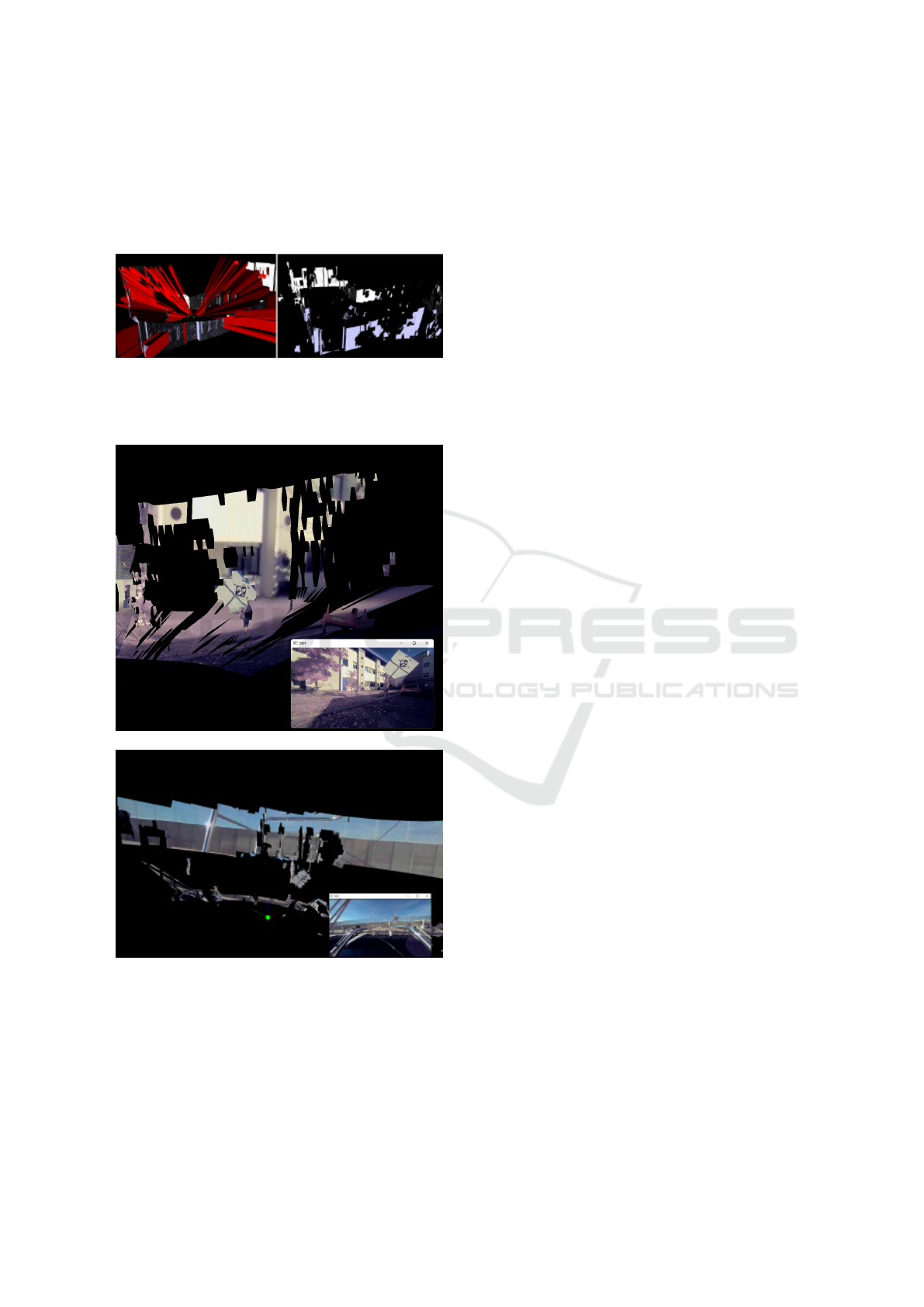
Figure 7: Elongated triangles (in red) usually connect por-
tions of surfaces that are disconnected/different and hence
automatically removed. The Left and right images show the
same data before and after removal of triangles.
Figure 8: Snapshots of the textured geometry. The camera
feed is also shown at the bottom.
Projecting RGB Images. The final color of the ge-
ometry is obtained by means of projective textur-
ing (NVidia, 2001). This requires a first rendering
pass where, for each camera, a shadow map is created
and used in the rendering pass to see from which cam-
eras each point is visible. Please note that, typically,
there are regions of space that are covered by mul-
tiple cameras, therefore we need an efficient way to
combine the, usually different, contributions in a rea-
sonable way. We use the technique presented in (Cal-
lieri et al., 2008) which consists of blending the con-
tribution of each camera according to the cosine of
the angle of the projection direction with the surface
normal. Furthermore, we apply an image equaliza-
tion step based on histogram matching (Pizer et al.,
1987) for a better blending of images in overlapping
regions.
Remote Rendering. The tessellated point cloud fol-
lowed by projective texturing based on the camera
vantage point generates a realistic rendering of the en-
vironment. The rendering data is directly read from
the GPU (framebuffer) and parsed as a stream of
jpeg images strictly maintaining the quality of the
rendered output. The remote rendering is facilitated
by a separate MJPEG streaming network socket con-
nection apart from our usual client-server communi-
cation. The MJPEG-encoded videos are then sent
over HTTP protocols using an easily integrable multi-
threaded and computationally inexpensive streaming
framework allowing clients to remotely visualize real-
time rendered content on a web browser. Besides the
MJPEG streaming, our application also supports vi-
sualization of the rendered content as H264 streams
over real-time streaming protocol(RTSP) using FFM-
PEG library (Tomar, 2006).
6 CONCLUSION
We presented a system for real-time acquisition and
rendering of 3D scenes using low-cost LIDARs and
RGB cameras, dubbed NausicaaVR. NausicaaVR
supports semi-automatic calibration, on-the-fly tes-
sellation, and remote rendering and is built with a
client-server architecture. A possible direction of im-
provement is the rendering of the reconstructed scene.
Although the results of our system were satisfactory
for the goal of environmental awareness, the regular
tessellation of the data creates several rendering arti-
facts, especially due to unsampled regions that cause
part of the images to be projected on the background.
One viable solution would be not to use the geome-
try as it is but as a proxy to place impostors,i.e, basic
primitive shapes onto which to project texture. How-
ever, the use of impostors should be combined with
real-time segmentation of the images in order to avoid
pixels belonging to the background (e.g. the sky) be-
ing projected into such impostors. Another avenue for
research is to use 3D data from multiple frames. With
On-the-Fly Acquisition and Rendering with Low Cost LiDAR and RGB Cameras for Marine Navigation
181

the current solution, each frame is rendered as is but
instead we could cumulate the point clouds from mul-
tiple frames for creating a more complete geometry.
However, since the boat is not steady, we would need
its position and orientation to place the data in a com-
mon reference system, that is, to compensate for the
motion and rotation. This information could be ob-
tained by using an IMU sensor, which unfortunately
was not available at this time.
ACKNOWLEDGEMENTS
This work was supported by the project NAUSICAA
- NAUtical Safety by means of Integrated Computer-
Assisted Appliances 4.0 (DIT.AD004.136)
REFERENCES
An, P., Ma, T., Yu, K., Fang, B., Zhang, J., Fu, W., and Ma,
J. (2020). Geometric calibration for lidar-camera sys-
tem fusing 3d-2d and 3d-3d point correspondences.
Opt. Express, 28(2):2122–2141.
Berger, M., Tagliasacchi, A., Seversky, L. M., Alliez, P.,
Guennebaud, G., Levine, J. A., Sharf, A., and Silva,
C. T. (2017). A survey of surface reconstruction from
point clouds. In Computer Graphics Forum, vol-
ume 36, pages 301–329. Wiley Online Library.
Brinkmann, M. and Hahn, A. (2017). Testbed architecture
for maritime cyber physical systems. In 2017 IEEE
15th International Conference on Industrial Informat-
ics (INDIN), pages 923–928.
Bu, Z., Sun, C., Wang, P., and Dong, H. (2021). Calibra-
tion of camera and flash lidar system with a triangular
pyramid target. Applied Sciences, 11(2).
Callieri, M., Cignoni, P., Corsini, M., and Scopigno, R.
(2008). Masked photo blending: mapping dense pho-
tographic dataset on high-resolution 3d models. Com-
puter & Graphics, 32(4):464–473. for the online ver-
sion: http://dx.doi.org/10.1016/j.cag.2008.05.004.
Corsini, M., Cignoni, P., and Scopigno, R. (2012). Efficient
and flexible sampling with blue noise properties of tri-
angular meshes. IEEE Transactions on Visualization
and Computer Graphics, 18(6):914–924.
dspace (2021). https://www.dspace.com/en/pub/home/
applicationfields/stories/smartkai-parking-assistance-
f.cfm.
Garrido-Jurado, S., Mu
˜
noz-Salinas, R., Madrid-Cuevas, F.,
and Mar
´
ın-Jim
´
enez, M. (2014). Automatic generation
and detection of highly reliable fiducial markers under
occlusion. Pattern Recognition, 47(6):2280–2292.
Hahn, T., Damerius, R., Rethfeldt, C., Schubert, A. U.,
Kurowski, M., and Jeinsch, T. (2022). Automated
maneuvering using model-based control as key to au-
tonomous shipping. at - Automatisierungstechnik,
70(5):456–468.
ImagingSource (2017). https://www.theimagingsource.
com.
Kim, H., Kim, D., Park, B., and Lee, S.-M. (2020). Arti-
ficial intelligence vision-based monitoring system for
ship berthing. IEEE Access, 8:227014–227023.
Li, Q., Queralta, J. P. n., Gia, T. N., Zou, Z., and West-
erlund, T. (2020). Multi-sensor fusion for navigation
and mapping in autonomous vehicles: Accurate local-
ization in urban environments. Unmanned Systems,
08(03):229–237.
Li, X., He, F., Li, S., Zhou, Y., Xia, C., and Wang, X.
(2022). Accurate and automatic extrinsic calibration
for a monocular camera and heterogenous 3d lidars.
IEEE Sensors Journal, 22(16):16472–16480.
Martelli, M., Virdis, A., Gotta, A., Cassar
`
a, P., and
Di Summa, M. (2021). An outlook on the future ma-
rine traffic management system for autonomous ships.
IEEE Access, 9:157316–157328.
NVidia (2001). https://www.nvidia.com/en-us/drivers/
Projective-Texture-Mapping/.
Nvidia (2017). Nvidia announces jetson tx2: Parker comes
to nvidia’s embedded system kit.
Paneque, J., Valseca, V., Mart
´
ınez-de Dios, J. R., and
Ollero, A. (2022). Autonomous reactive lidar-based
mapping for powerline inspection. In 2022 Inter-
national Conference on Unmanned Aircraft Systems
(ICUAS), pages 962–971.
Park, Y., Yun, S., Won, C. S., Cho, K., Um, K., and Sim, S.
(2014). Calibration between color camera and 3d lidar
instruments with a polygonal planar board. Sensors,
14(3):5333–5353.
Perera, L., Moreira, L., Santos, F., Ferrari, V., Sutulo, S.,
and Soares, C. G. (2012). A navigation and control
platform for real-time manoeuvring of autonomous
ship models. IFAC Proceedings Volumes, 45(27):465–
470. 9th IFAC Conference on Manoeuvring and Con-
trol of Marine Craft.
Pizer, S. M., Amburn, E. P., Austin, J. D., Cromartie, R.,
Geselowitz, A., Greer, T., ter Haar Romeny, B., Zim-
merman, J. B., and Zuiderveld, K. (1987). Adaptive
histogram equalization and its variations. Computer
vision, graphics, and image processing, 39(3):355–
368.
R
¨
ussmeier, N., Hahn, A., Nicklas, D., and Zielinski, O.
(2016). Ad-hoc situational awareness by optical sen-
sors in a research port maritime environment , ap-
proved networking and sensor fusion technologies.
Schiaretti, M., Chen, L., and Negenborn, R. R. (2017). Sur-
vey on autonomous surface vessels: Part i - a new de-
tailed definition of autonomy levels. In Bektas¸, T.,
Coniglio, S., Martinez-Sykora, A., and Voß, S., edi-
tors, Computational Logistics, pages 219–233, Cham.
Springer International Publishing.
Schubert, A. U., Kurowski, M., Gluch, M., Simanski, and
O Jeinsch, T. (2018). Manoeuvring automation to-
wards autonomous shipping. Zenodo.
Snyder, F. D., Morris, D. D., Haley, P. H., Collins, R. T.,
and Okerholm, A. M. (2004). Autonomous river nav-
igation. In SPIE Optics East.
GISTAM 2023 - 9th International Conference on Geographical Information Systems Theory, Applications and Management
182

Thombre, S., Zhao, Z., Ramm-Schmidt, H., Vallet Garc
´
ıa,
J. M., Malkam
¨
aki, T., Nikolskiy, S., Hammarberg,
T., Nuortie, H., H. Bhuiyan, M. Z., S
¨
arkk
¨
a, S., and
Lehtola, V. V. (2022). Sensors and ai techniques for
situational awareness in autonomous ships: A review.
IEEE Transactions on Intelligent Transportation Sys-
tems, 23(1):64–83.
Tomar, S. (2006). Converting video formats with ffmpeg.
Linux Journal, 2006(146):10.
Wright, R. G. (2019). Intelligent autonomous ship naviga-
tion using multi-sensor modalities. TransNav, the In-
ternational Journal on Marine Navigation and Safety
of Sea Transportation, 13(3):503–510.
On-the-Fly Acquisition and Rendering with Low Cost LiDAR and RGB Cameras for Marine Navigation
183