An Anisotropic and Asymmetric Causal Filtering Based Corner

Detection Method

Ghulam Sakhi Shokouh

, Philippe Montesinos

and Baptiste Magnier

EuroMov Digital Health in Motion, Univ. Montpellier, IMT Mines Ales, Ales, France

Keywords:

Causal Filter, Anisotropic Filtering, Asymmetric Diffusion, Corner Detection.

Abstract:

An asymmetric-anisotropic causal diffusion ﬁltering-based curvature operator is proposed in this communica-

tion. The new corner operator produces optimal results on small structures, such as, corners at pixel level and

also sub-pixel level precision. Meanwhile, this method is robust against noises due to its asymmetric diffusion

scheme. Experiments have been performed on a set of both synthetic and real images. The obtained results are

promising and better without any ambiguity as compared with the two referenced corner operators, namely

Kitchen Rosenfeld and Harris corner detector.

1 INTRODUCTION

The importance and interest in keypoint detection (i.e,

corner or junction as a stable interest point) in a digital

image lies notably in its application in image match-

ing, tracking, motion estimation, panoramic stitching,

object recognition, and 3D reconstruction (Schmid

et al., 2010). The reason for the corner detection’s

wide range of applications is that the corner is eas-

ier to localize than other low-level features such as

edges or lines, particularly taking into consideration

the correspondence problems (e.g., aperture problem

in matching). There are many corner detection tech-

niques based on classic handcrafted (Shokouh et al.,

2023) and deep learning methods (Wang et al., 2019).

Deep learning-based techniques are more automatic,

however, considering the accuracy and precision for

the detection of small structures, such as corners,

keypoints, etc., they do not generally present higher

performance (highly depends on the dataset quality,

and annotation which is not easy for small struc-

tures). We argue that handcrafted techniques are still

widely used, particularly for optimization purposes,

either independently or integrated into the prepro-

cessing or post-processing stages of machine learn-

ing based higher-level computer vision applications

(Junfeng et al., 2022). One of the example of com-

puter vision application that its performance directly

https://orcid.org/0000−0003−2561−7317

https://orcid.org/0000−0003−3741−8702

https://orcid.org/0000−0003−3458−0552

depends on the precision and accuracy of keypoint de-

tection is 3D reconstruction. Additionally, among the

classic handcrafted corner detection techniques, the

two corner detection operators Kitchen and Rosen-

feld (Kitchen and Rosenfeld, 1982), and Harris (Har-

ris and Stephens, 1988), are the main method used

for the comparison and benchmarking. Moreover,

Causal ﬁltering has proven its efﬁciency in many

segmentation domains, such as edge or line detec-

tion. In this contribution, we are presenting a new

segmentation method for corner detection based on

asymmetric anisotropic diffusion ﬁltering. The ba-

sic idea is inspired from a curvature-like operator

similar to the Kitchen-Rosenfeld operator, but imple-

mented through an asymmetric diffusion scheme us-

ing an anisotropic causal ﬁlter. Finally, we have com-

pared the experimental result of our operator with the

Kitchen and Rosen- feld, and Harris, the visual re-

sult presented higher precision for both pixel level and

sub-pixel level. The structure of this paper consists

of related works in the subsequent section, followed

by the proposed methods and the obtained result, and

eventually, the conclusion is presented.

2 RELATED WORKS

Considering a curve traced on the image plane, the

curvature is deﬁned as

dθ

where θ is the tangent to the

curve and s the curvilinear coordinate along the curve.

As an image, I(x, y) is a Cartesian parametrized sur-

Shokouh, G., Montesinos, P. and Magnier, B.

An Anisotropic and Asymmetric Causal Filtering Based Corner Detection Method.

DOI: 10.5220/0011855600003497

In Proceedings of the 3rd International Conference on Image Processing and Vision Engineering (IMPROVE 2023), pages 92-99

ISBN: 978-989-758-642-2; ISSN: 2795-4943

 2023 by SCITEPRESS – Science and Technology Publications, Lda. Under CC license (CC BY-NC-ND 4.0)

face as Eq. 1:

z = I(x y) (1)

An image can then be considered also as a set of

isophotes lines, at each pixel, there is in isophote line

going through this pixel. We can then deﬁne the dense

(at each pixel) the curvature of isophote lines in an

image is Eq. 2:

dθ

− 2I

+ I

)

(2)

This operator is the basis of the well-known corner

operator ”Kitchen-Rosenfeld” (Kitchen and Rosen-

feld, 1982) which is formed by the multiplication of

the curvature of isophotes lines and the norm of the

gradient. This formula means that a corner point must

be an edge point with a strong curvature. Then the Eq.

KR =

− 2I

+ I

)

(3)

It is also well-known that the Laplacian operator ap-

plied to an image can be written as Eq. 4:

∆I =

− 2I

+ I

)

+ 2I

+ I

)

(4)

Then as Eq. 5 :

∆I = I

+ I

= I

ξξ

+ I

ηη

(5)

It comes that I

ξξ

is the second derivative of the image

along the direction of the isophote ξ and I

ηη

is the

second derivative of the image along the direction of

the gradient η. As evidence, KR is equivalent to I

ξξ

The Harris and Stephen (Harris and Stephens, 1988)

proposed corner operator based on the structure tensor

as Eq. 6;

T =



) ∗ G



(6)

This structure tensor obtained from gradient tensor

represents the local auto-correlation of the image sig-

nal. I

and Y

are image derivatives along respectively

X and Y axis. They are obtained using a Gaussian

derivative ﬁlter with a σ

standard-deviation.

is a Gaussian smoothing ﬁlter with a σ

standard-

deviation.

Then the Harris operator is obtained from this tensor

as Eq. 7:

H = Det(T ) − k · Trace(T)

(7)

• The determinant is the product of eigen values, it

is strong when both eigen values are strong.

• The trace is the sum of eigen values and is strong

at edges.

• The parameter k has been determined empirically

to do a balance between corners and edges. k is

generally set to 0.04.

2.1 Diffusion Scheme

There are two important diffusion schemes.

• The Euclidean linear scale space :

This diffusion scheme is described by the Heat

equation, whose solution is a convolution of

the original image with a Gaussian. Then the

Kitchen-Rosenfeld operator can be seen as the

curvature multiplied by the gradient at a certain

level of diffusion.

• The Euclidean morphological scale space :

This non-linear scale-space is obtained by apply-

ing the Mean Curvature Motion (MCM) scheme

(Franke et al., 1996) Eq. 8.



I(0, x, y) = I

(x, y)

∂I

∂t

(t, x, y) = I

ξξ

(t, x, y)

(8)

Where ξ still represent the tangent to isophotes.

When iterating this scheme, isophote lines are

moving in function of their Euclidean curvature.

The Fig. 1 illustrates this property. If iterations

goes on, the rectangle will be changed to a circle

of decreasing radius.

(a) Initial image (b) MCM diffusion

Figure 1: MCM behavior. a) initial image, b) result of

MCM diffusion (100 iterations).

It is clear that such diffusion schemes are moving in

the corners as well as Gaussian scale space. In both

schemes, the I

ξξ

term is present.

3 PROPOSED METHOD

In this study we have used a completely different

scheme based on asymmetric diffusion ((Montesinos

and Magnier, 2017)) which corresponds exactly to our

An Anisotropic and Asymmetric Causal Filtering Based Corner Detection Method

needs of detecting corners precisely. Then we are go-

ing to show that one curvature-like measure that is

used to drive the numerical scheme provides a better

alternative to the I

ξξ

operator for corner detection.

3.1 An Asymmetric Diffusion Scheme

At each pixel P, ﬁve distinct directions are deﬁned:

• ξ

and ξ

are the direction deﬁned by the appli-

cation of a bank of ﬁrst derivative causal ﬁlters.

These directions are the direction given by the

smoothing component of the ﬁlter giving the ex-

ternal response (ξ

corresponds to the maximal

positive response, ξ

to the minimal negative one).

• ξ is the orientation of the tangent to the isophote.

This orientation is computed using ξ

and ξ

• ξ

and ξ

are the mirrored orientations of ξ

and

by the axis ξ (See Fig. 2a)).

This scheme can then be written as Eq. 9:







I(0, x, y) = I

(x, y) ← initial image

∂I

∂t

(t, x, y) = I

(t, x, y) = arg min

, I

ξξ

|x |

(9)

This scheme has a geometrical interpretation, illus-

trated at the Fig. 2. We have already seen that ori-

entations ξ

and ξ

are inﬂuenced by the presence of

edges, then at each pixel, we are searching for the di-

rections that are the less inﬂuenced by edges in order

to preserve these edges at most as possible by asym-

metric diffusion. The diffusion will be achieved along

ξ, along ξ

and ξ

, or along ξ

and ξ

, in respect to

the minimum absolute value of the asymmetric sec-

ond derivative of the image. In the conﬁguration of

Fig 2b), or Fig. 2c) the diffusion is applied in the

direction ξ

and ξ

, preserving the edges. On the

conﬁguration of Fig. 2a), the pixel under considera-

tion is located on an edge, the diffusion may be either

along ξ

and ξ

or simply along, ξ depending on the

local curvature. For this scheme, the only parameter

is the number of iterations.

For regularizing the input image, we just proceed

to several iterations of this asymmetric scheme (in

general, 100 iterations give good results). The Fig.

3 presents results of regularization obtained on the

“rectangle image” a), 3b) presents results obtained

with 100 iterations, 200 iterations at c) and 500 it-

erations at d). As we can see, corners are not affected

even with a high number of iterations.

3.2 Asymmetric Curvature

This scheme uses three curvature-like expressions to

perform the diffusion :

• |I

| :

a corner point is ﬁrst an edge point with a small-

est value of |I

| under a certain neighborhood

because ξ

and ξ

are both directions of isophotes

then, at the corner point location, the three gray-

levels involved in |I

| are similar.

• |I

ξξ

| :

this measure is similar to the Kitchen-Rosenfeld

measure (direction ξ may be somewhat different

because ﬁlters involved are different) estimated

locally in a 3 × 3 window. This measure is suit-

able but not optimal, the next measure will be pre-

ferred.

• |I

| :

this measure is maximized since the directions,

and ξ

indicates the directions where gray-

levels are the most different from the considered

pixel. For this reason, the response obtained is

less noisy than the one obtained with the preced-

ing measure.

Then, for characterizing the curvature at corner

points, we have chosen to use the expression |I

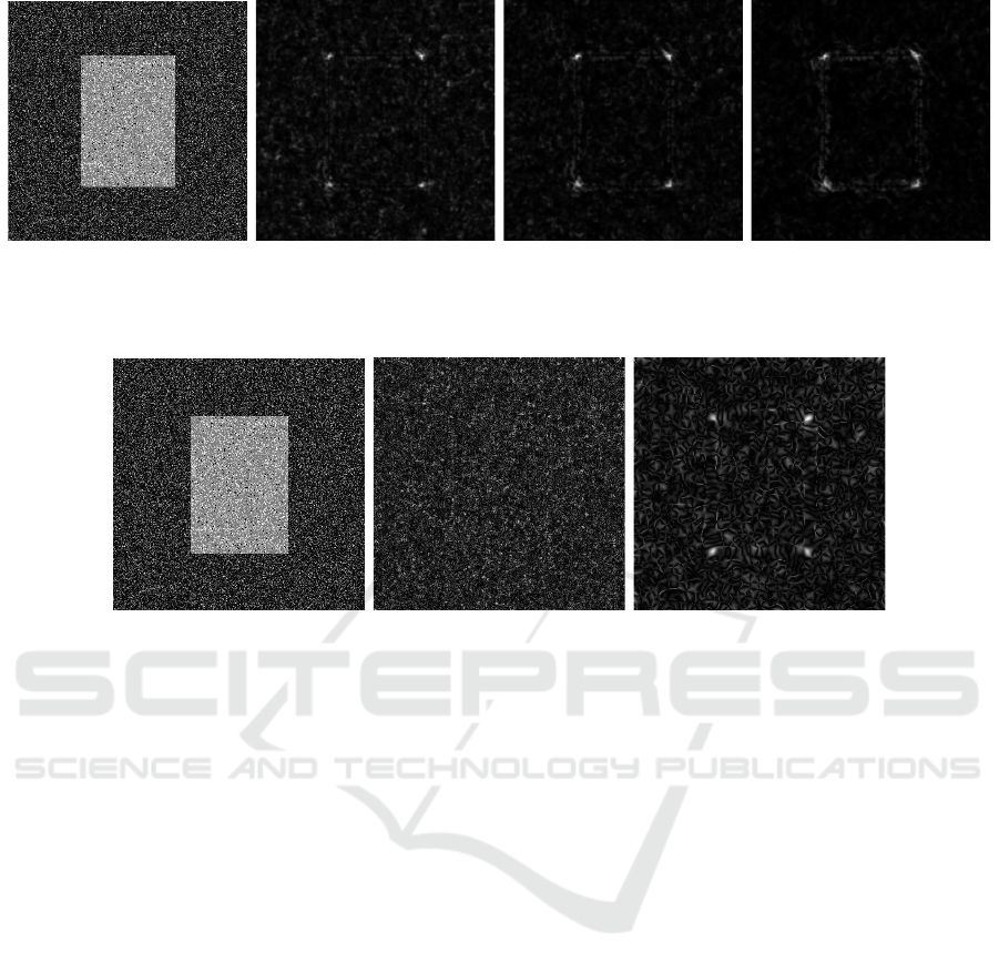
that best characterizes the corners. The Fig. 4

presents the three asymmetric curvature results ob-

tained after 100 iterations. As explained beforehand,

the |I

| (Fig. 4a)) gives 2 responses at each side of

corners. This measure is minimum at corner points,

for this reason it will be complicated to use such mea-

sure to characterize correctly corners. The |I

ξξ

| (Fig.

4b)) is similar to a Kitchen Rosenfeld measure, the

response is overall noisy and edges are also respond-

ing. Finally, the | I

| (Fig. 4c) measure gives the

best information able to characterize reliably the cor-

ner points.

3.3 Corner Detection Using | I

The complete algorithm for asymmetric corner detec-

tion is summarized as follows :

1. Depending on the precision needed, magnify or

not the initial image ((Montesinos and Datteny,

1997)) using a very small Gaussian standard-

deviation (σ ≃ 0.6), apply several iterations (in

general 10) of a heat inverse equation scheme then

apply several iterations (in general 4) of a shock

ﬁlter ((Osher and Rudin, 1990)).

2. Apply several iterations of the asymmetric

scheme (in general 100).

3. Compute the |I

| image after the regulariza-

tion.

4. Compute the local maxima of the |I

| for ex-

ample in a circular window (generally with a ra-

dius of 2 pixels multiplied by the precision).

IMPROVE 2023 - 3rd International Conference on Image Processing and Vision Engineering

edge edge

edge

Figure 7: Causal orientations.

a) b) c) d)

Figure 8: Asymetric regularization. a) initial image, b) asymetric regularization 100 iterations, c) asymetric

regulariz a tio n 200 iterations, d) asymetric regularization 500 iterat ions .

3.1.3 Asymetric curvature

This scheme uses three curvatur e -li ke expressions to perform the diﬀusion :

• |I

a corner point is ﬁrst an edge point with a smallest value of |I

| u n de r a cer tain neighborh ood because

and ξ

are both directions of isophotes then, at the corner point location, the three grey levels involved

in |I

| are similar.

• |I

ξξ

this measure is similar to th e Kitchen-Rosenfeld measure (direction ξ may be somewhat diﬀerent because

ﬁlters involved are diﬀerent) estimated locally in a 3×3 window. This measure is suitable but not optimal,

next measure will be prefered.

• |I

this measure is maximized since the dire cti ons ξ

and ξ

indicates the directions where grey levels are

the most diﬀerent from the considered pixel. For this reason the re s ponse obtained is less noisy that the

one obtained with the preceding measure.

Then f or characterizing the curvature at corner points, we have choosen to use the expression |I

| t hat

best characterizes the corners. The ﬁgure 9 presents the three asymetric curvature results obtained after 100

iterations. As explained precedently the |I

| (ﬁgure 9a)) gives 2 responses at each side of corners. This

measure is minimum at corner points, for this reason it will be complicated to use such measure to characterize

correctly corners. The |I

ξξ

| (ﬁgure 9b)) is similar to a Kitchen r os en fakd mesure, the response is averall noisy

and edges are also responding.

Finally the |I

| (ﬁgur e 9c)) measure gives the best information able to characterize reliably the corner

points.

edge edge

edge

Figure 7: Causal orientations.

a) b) c) d)

Figure 8: Asymetric regularization. a) initial image, b) asymetric regularization 100 iterations, c) asymetric

regulariz a tio n 200 iterations, d) asymetric regularization 500 iterat ions .

3.1.3 Asymetric curvature

This scheme uses three curvatur e -li ke expressions to perform the diﬀusion :

• |I

a corner point is ﬁrst an edge point with a smallest value of |I

| u n de r a cer tain neighborh ood because

and ξ

are both directions of isophotes then, at the corner point location, the three grey levels involved

in |I

| are similar.

• |I

ξξ

this measure is similar to th e Kitchen-Rosenfeld measure (direction ξ may be somewhat diﬀerent because

ﬁlters involved are diﬀerent) estimated locally in a 3×3 window. This measure is suitable but not optimal,

next measure will be prefered.

• |I

this measure is maximized since the dire cti ons ξ

and ξ

indicates the directions where grey levels are

the most diﬀerent from the considered pixel. For this reason the re s ponse obtained is less noisy that the

one obtained with the preceding measure.

Then f or characterizing the curvature at corner points, we have choosen to use the expression |I

| t hat

best characterizes the corners. The ﬁgure 9 presents the three asymetric curvature results obtained after 100

iterations. As explained precedently the |I

| (ﬁgure 9a)) gives 2 responses at each side of corners. This

measure is minimum at corner points, for this reason it will be complicated to use such measure to characterize

correctly corners. The |I

ξξ

| (ﬁgure 9b)) is similar to a Kitchen r os en fakd mesure, the response is averall noisy

and edges are also responding.

Finally the |I

| (ﬁgur e 9c)) measure gives the best information able to characterize reliably the corner

points.

edge edge

edge

Figure 7: Causal orientations.

a) b) c) d)

Figure 8: Asymetric regularization. a) initial image, b) asymetric regularization 100 iterations, c) asymetric

regulariz a tio n 200 iterations, d) asymetric regularization 500 iterat ions .

3.1.3 Asymetric curvature

This scheme uses three curvatur e -li ke expressions to perform the diﬀusion :

• |I

a corner point is ﬁrst an edge point with a smallest value of |I

| u n de r a cer tain neighborh ood because

and ξ

are both directions of isophotes then, at the corner point location, the three grey levels involved

in |I

| are similar.

• |I

ξξ

this measure is similar to th e Kitchen-Rosenfeld measure (direction ξ may be somewhat diﬀerent because

ﬁlters involved are diﬀerent) estimated locally in a 3×3 window. This measure is suitable but not optimal,

next measure will be prefered.

• |I

this measure is maximized since the dire cti ons ξ

and ξ

indicates the directions where grey levels are

the most diﬀerent from the considered pixel. For this reason the re s ponse obtained is less noisy that the

one obtained with the preceding measure.

Then f or characterizing the curvature at corner points, we have choosen to use the expression |I

| t hat

best characterizes the corners. The ﬁgure 9 presents the three asymetric curvature results obtained after 100

iterations. As explained precedently the |I

| (ﬁgure 9a)) gives 2 responses at each side of corners. This

measure is minimum at corner points, for this reason it will be complicated to use such measure to characterize

correctly corners. The |I

ξξ

| (ﬁgure 9b)) is similar to a Kitchen r os en fakd mesure, the response is averall noisy

and edges are also responding.

Finally the |I

| (ﬁgur e 9c)) measure gives the best information able to characterize reliably the corner

points.

(a) Pixel located on an edge (b) Pixel located outside edge (c) Pixel located inside edge

Figure 2: Causal Orientation. a) The pixel is located on an edge, the diffusion may be either along ξ

and ξ

, b) Pixel is

outside edge and the diffusion is applied in the direction ξ

and ξ

, preserving the edges, c) Pixel is inside edge and the

diffusion is applied in the direction ξ

and ξ

, preserving the edges.

(a) Initial image (b) Regularization 100 iterations (c) Regularization 200 iterations (d) Regularization 500 iterations

Figure 3: Asymmetric regularization. a) initial image, b) asymmetric regularization 100 iterations, c) asymmetric regulariza-

tion 200 iterations, d) asymmetric regularization 500 iterations.

(a) |I

| (b) |I

ξξ

| (c) |I

(d) Original image (e) |I

| measures (f) |I

ξξ

| measures (g) |I

| measures

Figure 4: Anisotropic curvature measures obtained after 100 iterations. a) | I

|, b) | I

ξξ

|, c) | I

|. d), e), f), g) Details in

the upper left corner (d) original image) e, f, g) respectively |I

|, |I

ξξ

|, and |I

| measures.

An Anisotropic and Asymmetric Causal Filtering Based Corner Detection Method

(a) Original image (b) |I

| at 100 iterations (c) |I

| at 200 iterations (d) |I

| at 500 iterations

Figure 5: Asymmetric curvature | I

| on image ”rectangle”. a) original image, b) |I

| at 100 iterations, c) |I

| at

200 iterations, d) |I

| at 500 iterations.

(a) Original image (b) Kitchen-Rosenfeld (σ = 1) (c)Kitchen-Rosenfeld (σ = 3)

Figure 6: Kitchen-Rosenfeld operator on image ”rectangle”. a) original image, b) Kitchen-Rosenfeld (σ = 1) regularization is

not enough to obtain reliable curvature, c) Kitchen-Rosenfeld (σ = 3) curvature appears, but noise is still present and strong.

4 RESULT

The Fig.5 presents the | I

| operator results ob-

tained on the “rectangle” image at simple pixel pre-

cision, after varying number of iterations (100, 200,

500). As iterations go on, the noise is ﬁltered.

For comparison, the Fig. 6 presents the Kitchen-

Rosenfeld operator results obtained with a Gaussian

standard-deviation σ = 1 and σ = 3. The Kitchen-

Rosenfeld operator gives noisy results. When com-

puted with a Gaussian ﬁlter having a parameter σ

equal to 1 the results obtained are generally too noisy

to obtain interesting results (Fig. 6b)). If the parame-

ter σ increases, it is possible to obtain a more reliable

information, but local maxima are moving (Fig. 6c)).

Finally, the Fig. 7 present results obtained by local

maxima extraction for all operators : Harris (σ = 1),

Kitchen-Rosenfeld (σ = 3) and |I

| with 100, 200

and 500 iterations. As discussed beforehand, Harris

and Kitchen-Rosenfeld give noisy results. Moreover,

for Kitchen-Rosenfeld, corners are often detected at

a distance greater than 2 pixels from the true loca-

tion. Increasing the Gaussian parameter σ improves

the curvature SNR (signal-to-noise ratio), but preci-

sion of corner localization decreases. Concerning the

| operator, the response is less noisy, and the

precision seems better than Harris (around 1 pixel

from the true corner locations).

The Fig. 8 compares the Harris operator and the

anisotropic curvature operator on the ”inria” image :

a) shows the initial image, b) presents regularization

results (100 iterations) and c) presents the |I

operator result. The Fig. 8 b) and c) show respec-

tively the results of the Harris corner detector and the

| corner detection. Then the Fig. 8 d) present

4 manually corner selection and the results obtained

with both operators are going to be detailed in Fig. 8

e). For the Fig. 8 e), for those corner angle which is

less or equal to 90

◦

, the new operator performs bet-

ter than Harris, and for those corner angle which is

108

◦

(angle is wider) the results are similar. But if

angle value increases Harris completely lost the cor-

ner point, The new operator still performs correctly

(see the wide angles of the black carpet corners on

the ﬂoor).

4.1 Sub-pixel Precision

The Fig. 9 compares Harris corner detector (thresh-

old=0.001) and | I

| corner detection (thresh-

IMPROVE 2023 - 3rd International Conference on Image Processing and Vision Engineering

(a) Original image (b) Harris (c) Kitchen-Rosenfeld

(d) Anisotropic (100 iteration) (e) Anisotropic (200 iteration) (f) Anisotropic (500 iteration)

Figure 7: Corner detection. a) Harris corner detector (threshold = 0.1), b) Kitchen-Rosenfeld corner detector (σ = 3, thresh-

old=0.3), c) Anisotropic corner detector (100 iterations, threshold = 0.3), d) Anisotropic corner detector (200 iterations,

threshold = 0.3), e) Anisotropic corner detector (500 iterations, threshold = 0.3.

old=0.05) at pixel precision. We are interested here

on the results obtained on the small windows of the

central house (windows size is around 5 × 5 pixels).

Harris operator (Fig. 9 b)) gives many responses on

the windows, but the points detected are often on the

windows frame rather than the corner. For the |I

(Fig. 9 c)) corner detection, the detected point is more

often at the corner. On the large, dark windows of the

left house, Harris performs better.

The Fig. 10 present results obtained at preci-

sion=2 (

pixel). In 10 a) are presented the sub-pixel

(

pixel) Harris corner detector, and in 10 b) are pre-

sented the sub-pixel (

pixel) |I

| corner detector.

The Fig. 10 c) and d) present the details only a region

of interest 200 × 200 on the windows of the central

house (c) Harris, d) |I

5 CONCLUSIONS

This paper presents an asymmetric diffusion-based

anisotropic causal corner operator. The proposed

approach presented higher precision and accuracy

than the compared well-known corner detectors, such

as Kitchen Rosenfeld and Harris and Stephen tech-

niques, which are known as a reference benchmarks.

Meanwhile, to better regularize the image and im-

prove the robustness against noises, an asymmetric

diffusion scheme is used. The experimental results

on synthetic images and real images, both on pixel

and subpixel precision, validate visually the perfor-

mance of our method. This work can particularly

contribute to applications that require keypoint detec-

tion with higher precision, such as 3D reconstruction

(Peng et al., 2009), object detection, etc. Correspond-

ingly, as the outlook of this work will be to examine

this technique for the 3D reconstruction and then pur-

sue an objective evaluation (Shokouh et al., 2023).

REFERENCES

Franke, T., Neumann, H., and Seydel, R. (1996).

Anisotropic diffusion based on mean curvature mo-

tion: A computational study. In J

ahne, B., Geißler, P.,

Haußecker, H., and Hering, F., editors, Mustererken-

nung 1996, pages 47–54, Berlin, Heidelberg. Springer

Berlin Heidelberg.

Harris, C. G. and Stephens, M. J. (1988). A combined cor-

ner and edge detector. In Alvey Vision Conference,

pages 147–151.

Junfeng, J., Shenjuan, L., Gang, W., Weichuan, Z., and

Changming, S. (2022). Recent advances on image

edge detection: A comprehensive review. Neurocom-

puting.

An Anisotropic and Asymmetric Causal Filtering Based Corner Detection Method

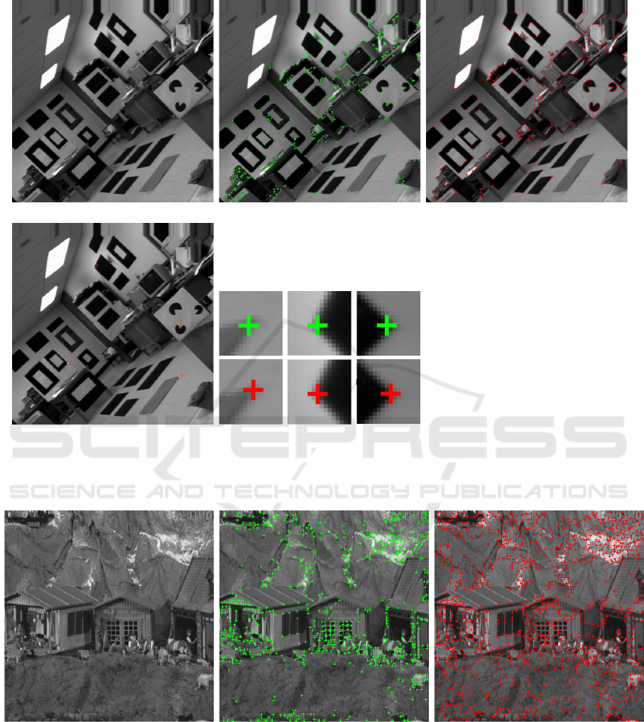
(a) Original image (b) Harris (c) Proposed anisotropic

(d) Corner locations highlighted (e) Corner (424, 390),(209, 112), (140, 355) of d

Figure 8: Corner detection on the image ”inria”. a) Original image, b) Harris corner detection operator (threshold = 0.001)

, c) Anisotropic corner detection operator (threshold = 0.1). d) Few detected corner highlighted. e) Comparative corner

precision at location(424, 390),(209, 112), (140, 355) highlighted in d).

(a) Initial image (b) Harris (c) Proposed anisotropic

Figure 9: Corner detection image ”toys”, pixel precision. a) initial image. b) Harris corner detector (threshold = 0.001), c)

Anisotropic corner detector (threshold = 0.05).

IMPROVE 2023 - 3rd International Conference on Image Processing and Vision Engineering

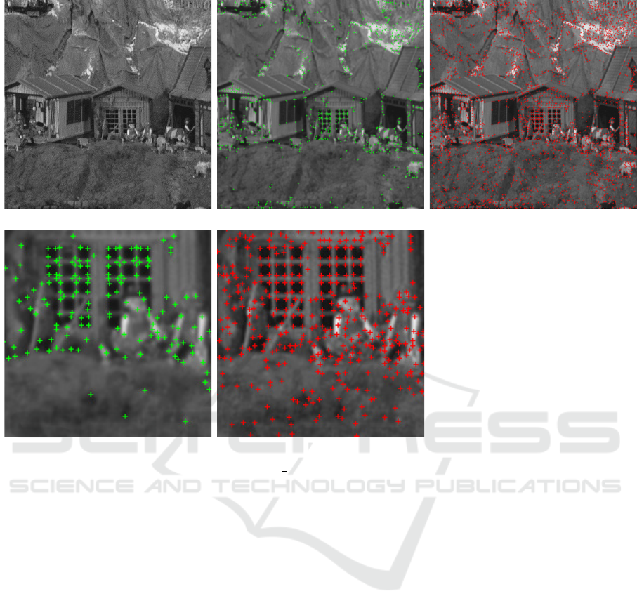
(a) Original image (b) Harris (c) Proposed anisotropic

(d) Harris (window details) (e) Proposed (window details)

Figure 10: Corner detection image ”toys”, precision =

pixel. a) Harris corner detector (threshold = 0.001), b) Anisotropic

corner detector (threshold = 0.05), c) Harris corner detector (window details), d) Anisotropic corner detector (window details).

Kitchen, L. and Rosenfeld, A. (1982). Gray-level corner

detection. Pattern Recognit. Letters, 1:95–102.

Montesinos, P. and Datteny, S. (1997). Sub-pixel accuracy

using recursive ﬁltering. In Scandinavian Conference

on Image Analysis.

Montesinos, P. and Magnier, B. (2017). Des ﬁltres

anisotropes causaux pour une diffusion non con-

trolled. In GRETSI.

Osher, S. and Rudin, L. (1990). Feature-oriented image en-

hancement using shock ﬁlter. In SIAM Journal of Nu-

merical Analysis.

Peng, K., Chen, X., Zhou, D., and Liu, Y. (2009). 3d re-

construction based on sift and harris feature points. In

2009 IEEE International Conference on Robotics and

Biomimetics (ROBIO), pages 960–964.

Schmid, C., Mohr, R., and Bauckhage, C. (2010). Evalua-

tion of interest point detectors. IJCV, 37:151–172.

Shokouh, G.-S., Montesinos, P., and Magnier, B. (2023).

Repeatability evaluation of keypoint detection tech-

niques in tracking underwater video frames. In

CVAUI, to appear. Springer Berlin Heidelberg.

Wang, L., Han, K., and Sun, H. (2019). An adap-

tive corner detection method based on deep learning.

In 2019 Chinese Control Conference (CCC), pages

8478–8482.

An Anisotropic and Asymmetric Causal Filtering Based Corner Detection Method