Learning Less Generalizable Patterns for Better Test-Time Adaptation

Thomas Duboudin

, Emmanuel Dellandr

, Corentin Abgrall

, Gilles H

enaff

and Liming Chen

Univ. Lyon,

Ecole Centrale de Lyon, CNRS, INSA Lyon, Univ. Claude Bernard Lyon 1,

Univ. Louis Lumi

ere Lyon 2, LIRIS, UMR5205, 69134 Ecully, France

Thales LAS France SAS, 78990

Elancourt, France

Keywords:

Domain Generalization, Out-of-Domain Generalization, Test-Time Adaptation, Shortcut Learning, PACS,

Ofﬁce-Home.

Abstract:

Deep neural networks often fail to generalize outside of their training distribution, particularly when only a

single data domain is available during training. While test-time adaptation has yielded encouraging results in

this setting, we argue that to reach further improvements, these approaches should be combined with training

procedure modiﬁcations aiming to learn a more diverse set of patterns. Indeed, test-time adaptation methods

usually have to rely on a limited representation because of the shortcut learning phenomenon: only a subset of

the available predictive patterns is learned with standard training. In this paper, we ﬁrst show that the combined

use of existing training-time strategies and test-time batch normalization, a simple adaptation method, does

not always improve upon the test-time adaptation alone on the PACS benchmark. Furthermore, experiments

on Ofﬁce-Home show that very few training-time methods improve upon standard training, with or without

test-time batch normalization. Therefore, we propose a novel approach that mitigates the shortcut learning

behavior by having an additional classiﬁcation branch learn less predictive and generalizable patterns. Our

experiments show that our method improves upon the state-of-the-art results on both benchmarks and beneﬁts

the most to test-time batch normalization.

1 INTRODUCTION

Deep neural networks’ performance falls sharply

when confronted, at test-time, with data coming from

a different distribution (or domain) than the training

one. A change in lighting, sensor, weather conditions

or geographical location can result in a dramatic per-

formance drop (Hoffman et al., 2018; Beery et al.,

2018; DeGrave et al., 2021). Such environmental

changes are commonly encountered when an embed-

ded network is deployed in the wild and exist in such

diversity that it is impossible to gather enough data to

cover all possible domain shifts. This lack of cross-

domain robustness prevents the widespread deploy-

ment of deep networks in safety-critical applications.

Domain generalization algorithms have been investi-

gated to mitigate the test-time performance drop by

modifying the training procedure. Contrary to the do-

main adaptation research ﬁeld, no information about

the target domain is assumed to be known in domain

generalization. Most of the existing works assume to

have access to data coming from several identiﬁed dif-

ferent domains and try to create a domain invariant

representation by ﬁnding common predictive patterns

(Li et al., 2018b; Moyer et al., 2018; Carlucci et al.,

2019; Li et al., 2018a; Krueger et al., 2020; Huang

et al., 2020). However, such an assumption is quite

generous, and in many real-life applications, one does

not have access to several data domains but only a sin-

gle one. As a result, some works study single-source

domain generalization (Wang et al., 2021b; Shi et al.,

2020; Zhao et al., 2020; Zhang et al., 2022b; Nam

et al., 2021). However, most methods were found

to perform only marginally better than the standard

training procedure when the evaluation is done rigor-

ously on several benchmarks (Gulrajani and Lopez-

Paz, 2021; Zhang et al., 2022a). Another recent

paradigm, called test-time adaptation, proposes to use

a normally trained network and adapt it with a quick

procedure at test-time, using only a batch of unlabeled

target samples. This paradigm yielded promising re-

sults in the domain generalization setting (You et al.,

2021; Yang et al., 2022) because they alleviate the

main challenges of domain generalization: the lack of

information about the target domain and the require-

ment to be simultaneously robust in advance to every

possible shift.

However, test-time adaptation methods suffer

Duboudin, T., Dellandréa, E., Abgrall, C., Hénaff, G. and Chen, L.

Learning Less Generalizable Patterns for Better Test-Time Adaptation.

DOI: 10.5220/0011893800003417

In Proceedings of the 18th International Joint Conference on Computer Vision, Imaging and Computer Graphics Theory and Applications (VISIGRAPP 2023) - Volume 5: VISAPP, pages

349-358

ISBN: 978-989-758-634-7; ISSN: 2184-4321

 2023 by SCITEPRESS – Science and Technology Publications, Lda. Under CC license (CC BY-NC-ND 4.0)

349

from a drawback that limits their adaptation capabil-

ity, and which can only be corrected at training-time.

Indeed, using a standard training procedure, only a

subset of predictive patterns is learned, corresponding

to the most obvious and efﬁcient ones, while the less

predictive patterns are disregarded entirely (Singla

et al., 2021; Hermann and Lampinen, 2020; Pezeshki

et al., 2020; Hermann et al., 2020; Shah et al., 2020;

Beery et al., 2018; Geirhos et al., 2020). This appar-

ent ﬂaw, named shortcut learning, originates from the

gradient descent optimization (Pezeshki et al., 2020)

and prevents a test-time method from using all the

available patterns. The combination of a training-

time patterns diversity-seeking approach with a test-

time adaptation method may thus lead to improved

results. In this paper, we show that the combined use

of test-time batch normalization with the state-of-the-

art single-source domain generalization methods does

not systematically yield increased results on the PACS

benchmark (Li et al., 2017) in the single-source set-

ting, despite them being designed to seek normally ig-

nored patterns. Similar experiments on Ofﬁce-Home

(Venkateswara et al., 2017) yield a similar result, with

only a few methods performing better than the stan-

dard training procedure.

We thus propose a new method, called L2GP,

which encourages a network to learn more semanti-

cally different predictive patterns than the standard

training procedure. To ﬁnd such different patterns, we

propose to look for predictive patterns that are less

predictive than the naturally learned ones. By deﬁ-

nition, these patterns enable correct predictions on a

subset of the training data but not on all the others

and are, thus, less generalizable on the training dis-

tribution. These less generalizable patterns match the

ones normally ignored because of the simplicity bias

of deep networks that promotes the learning of a rep-

resentation with a high generalization capability on

the training distribution (Huh et al., 2021; Galanti and

Poggio, 2022). Our method requires two classiﬁers

added to a features extractor. They are trained asym-

metrically: one is trained normally (with the stan-

dard cross-entropy classiﬁcation loss only), and the

other with both a cross-entropy loss and an additional

shortcut avoidance loss. This loss slightly encourages

memorization rather than generalization by learning

batch-speciﬁc patterns, i.e. patterns that lower the loss

on the running batch but with a limited effect on the

other batches of data. The features extractor is trained

with respect to both classiﬁcation branches.

To summarize, our contribution is threefold:

• To the best of our knowledge, we are the ﬁrst to in-

vestigate the effect of training-time single-source

methods on a test-time adaptation strategy. We

show that it usually does not increase performance

and can even have an adverse effect.

• We apply, for the ﬁrst time, several state-of-the-art

single-source domain generalization algorithms

on the more challenging and rarely used Ofﬁce-

Home benchmark and showed that very few yield

a robust cross-domain representation.

• We propose an original algorithm to learn a larger

than usual subset of predictive features. We show

that it yields results competitive or over the state-

of-the-art with the combination of test-time batch

normalization.

Figure 1: Schema of our bi-headed architecture. The nam-

ing convention is the same as the one used in algorithm 1.

2 RELATED WORKS

2.1 Single-Source Domain

Generalization

Most domain generalization algorithms require sev-

eral identiﬁed domains to enforce some level of dis-

tributional invariance. Because this is an unrealistic

hypothesis in some situations (such as in healthcare

or defense-related tasks), methods were developed to

deal with a domain shift issue with only one single

domain available during training. Some of them rely

on a domain shift invariance hypothesis. A commonly

used invariance hypothesis is the texture shift hypoth-

esis. Indeed, many domain shifts are primarily tex-

tures shifts, and using style-transfer-based data aug-

mentation will improve the generalization. It can be

done explicitly by training a model on stylized im-

ages (Wang et al., 2021b; Jackson et al., 2019) or im-

plicitly in the internal representation of the network

(Zhang et al., 2022b; Nam et al., 2021). Such meth-

ods are limited to situations where it is indeed a shift

of the hypothesized nature that is encountered. Oth-

ers wish to learn a larger set of predictive patterns to

make the network more robust should one or several

training-time predictive patterns be missing at test-

VISAPP 2023 - 18th International Conference on Computer Vision Theory and Applications

350

Algorithm 1: Learning Less Generalizable Patterns (L2GP).

1 Method speciﬁc hyper-parameters:

2 - weight for the shortcut avoidance loss α

3 - step size used for the gradient perturbation lr

4 Networks:

5 - features extractor f , and its weights W (ResNet18 without its last linear layer)

6 - ﬁrst classiﬁer c

(single linear layer)

7 - second classiﬁer c

(single linear layer)

8 while training is not over do

9 sample 2 batches of data {(x

, y

), i = 0...N − 1}, {(˜x

, ˜y

), i = 0...N − 1}

10 calculate the cross-entropy loss L on the ﬁrst batch for both branches on the original weights W :

11 L ( f , c

) =

∑

L [c

( f (W, x

)), y

]

12 L ( f , c

) =

∑

L [c

( f (W, x

)), y

]

13 calculate the gradient of the cross-entropy loss L w.r.t W on the ﬁrst batch:

14 ∇

L = ∇

∑

L [c

( f (W, x

)), y

]

15 add the perturbation to the running weight W , and track this addition in the computational graph:

16 W

= W + lr

∇

17 calculate the shortcut avoidance loss on the second batch:

18 L

( f , c

) =

∑

||c

( f (W, ˜x

)) − c

( f (W

, ˜x

))||

19 update all networks to minimize L

total

( f , c

, c

) =

(L ( f , c

) + L ( f , c

)) + αL

( f , c

)

20 end

21 At test-time: use c

◦ f (discard c

) combined with test-time batch normalization

time. (Volpi et al., 2018) and (Zhao et al., 2020) pro-

pose to incrementally add adversarial images crafted

to maximize the classiﬁcation error of the network to

the training dataset. These images no longer contain

the original obvious predictive patterns, which then

forces the learning of new patterns. These strategies

are inspired by adversarial training methods (Huang

et al., 2015; Kurakin et al., 2016) that were originally

designed to improve adversarial robustness in deep

networks. (Wang et al., 2021b) used a similar ap-

proach in an online fashion, without the impractical

ever-growing training dataset, and combined it with

a style augmentation approach. (Huang et al., 2020)

and (Shi et al., 2020) used a dropout-based (Srivas-

tava et al., 2014) strategy to prevent the network from

relying only on the most predictive patterns by mut-

ing the most useful channels or mitigating the texture

bias. These methods were evaluated in the single-

source setting on several benchmarks, including the

very common PACS dataset.

2.2 Test-Time Adaptation

Test-time adaption has emerged as a promising

paradigm to deal with domain shifts. Waiting to

gather information about the target domain, in the

shape of an unlabeled batch of samples (or even a

single sample), alleviates the main drawbacks of

training-time domain generalization methods: the

lack of information about the target domain, and

the necessity to simultaneously adapt to all possible

shifts. The simplest test-time adaptation strategy

consists of replacing the training-time statistics in the

batch normalization layers with the running test batch

statistics. It is now a mandatory algorithm block for

almost all methods (Nado et al., 2020; Benz et al.,

2021; You et al., 2021; Hu et al., 2021; Schneider

et al., 2020). This strategy was originally designed

to deal with test-time image corruptions but proved

to be efﬁcient in a more general domain shift setting

(You et al., 2021; Yang et al., 2022). In a situation

where samples of a test batch cannot be assumed

to come from the same distribution, workarounds

requiring a single sample were developed by mixing

test-time and training-time statistics (You et al.,

2021; Yang et al., 2022; Hu et al., 2021; Schneider

et al., 2020), or by using data augmentation (Hu

et al., 2021). Some solutions, such as the work of

(Yang et al., 2022) or (Wang et al., 2021a), further

rely on test-time entropy minimization to remove

inconsistent features from the prediction. Finally,

(Zhang et al., 2021) quickly adapt a network to make

consistent predictions between different augmenta-

tions of the same test sample. All these strategies

rely on a model trained with the standard training

procedure.

Learning Less Generalizable Patterns for Better Test-Time Adaptation

351

3 METHOD

Our approach requires two classiﬁcation layers

plugged after the same features extractor: one will

be tasked with learning the patterns that are nor-

mally learned (as they are not necessarily spurious

and, therefore, should not be systematically ignored),

and the other the normally ”hidden” ones. This

lightweight modiﬁcation of the standard architecture,

illustrated in ﬁgure 1, is compatible with many net-

works and tasks. The primary branch, consisting

in the features extractor and the primary classiﬁer,

is trained to minimize the usual cross-entropy loss

(algo.1, lines 11). The secondary one is trained

to minimize the cross-entropy loss (algo.1, line 12)

alongside a novel shortcut avoidance loss. The com-

plete procedure is available in algorithm 1.

If we are able to update a model in a direction

that lowers the loss value on a certain batch of data,

but does not produce a similar decrease on another

batch of the same distribution, it means that the pat-

terns learned are both predictive as they lower the

loss and generalize poorly, i.e. they are less predic-

tive. These are precisely the patterns we are look-

ing for. Our shortcut avoidance loss follows this idea.

We ﬁrst compute a new set of weights for the sec-

ondary branch by applying a single cross-entropy gra-

dient ascent step to the branch weights (algo.1, lines

13-16). The gradient is computed on the original run-

ning batch, already used for the cross-entropy losses.

We, then, compare the predictions of the secondary

branch with the current weights and the computed al-

tered weights (algo.1, lines 17-18). This difference in

predictions constitutes our shortcut avoidance loss.

Our approach requires the sampling of two

batches of data simultaneously because the shortcut

avoidance loss is computed on a batch of data differ-

ent from the one used to compute the applied gradient.

As the features learned in the applied gradient gener-

alize from one batch of data to the other, the altered

weights’ predictions are a lot less accurate than the

running weights’ predictions (cross-entropy gradient

ascent). As a result, these predictions differ greatly.

By training the secondary branch to minimize the gap

between both predictions, we are pushing the weights

toward an area in which the applied gradient does not

change the network’s secondary output. This would

mean that the patterns extracted for the second batch

are different from the ones learned in the applied gra-

dient. By adding the cross-entropy loss to the train-

ing procedure, we are driving the network to learn

weights that are both predictive for the running clas-

siﬁcation batch but that have a low effect on the pre-

dictions of another batch and are, hence, less predic-

tive. Note that the running network’s weights are opti-

mized with regard to both sides of the shortcut avoid-

ance loss. The addition of the gradient must thus be

tracked in the computational graph. This is akin to the

MAML (Finn et al., 2017) meta-learning framework

in which the starting point of a few optimization steps

is itself optimized.

During the evaluation, only the ﬁrst classiﬁer is

used, and the secondary one can be discarded. In-

deed, the ﬁrst classiﬁer uses every available feature at

its disposal, including those learned by the secondary

branch, while the secondary branch only favors less

simple features. Furthermore, we use test-time batch

normalization (abbreviated as TTBN). This method

has been chosen because of its simplicity and its wide

range of applicability. We do not use the usual expo-

nential average training mean and standard deviation

(computed during training) in the batch normalization

layers. Instead, we ﬁrst calculate the statistics on the

running test batch and use them to update an expo-

nential average of the test statistics, as in (Nado et al.,

2020; Benz et al., 2021; You et al., 2021; Hu et al.,

2021; Schneider et al., 2020), before using this esti-

mate to normalize the features. A correct target statis-

tics approximation can be reached only if all samples

encountered at test-time come from the same data dis-

tribution. This is a realistic scenario for applications

like autonomous driving, in which the data distribu-

tion is not expected to change over the course of a

few consecutive images. Several methods (You et al.,

2021; Hu et al., 2021) provide ways to circumvent

this issue if needed.

4 EXPERIMENTS AND RESULTS

4.1 Baselines for Comparison and

Experimental Setup

We compare our approach with the standard train-

ing procedure (expected risk minimization, abbrevi-

ated ERM), with several methods designed for single-

source domain generalization (Wang et al., 2021b;

Zhang et al., 2022b; Nam et al., 2021; Volpi et al.,

2018; Zhao et al., 2020; Shi et al., 2020), with Spec-

tral Decoupling (Pezeshki et al., 2020), a method de-

signed to reduce the shortcut-learning phenomenon in

deep networks, and with RSC (Huang et al., 2020),

and InfoDrop (Shi et al., 2020), that are domain gen-

eralization algorithms which do not explicitly require

several training domains. These baselines were se-

lected because they yield state-of-the-art results, are

representative of the main ideas in the single-source

domain generalization research community, and be-

VISAPP 2023 - 18th International Conference on Computer Vision Theory and Applications

352

Table 1: Performances of our approach and comparison with the state-of-the-art.

without TTBN with TTBN

Method Avg. Val. Acc. Avg. Test Acc. Avg. Val. Acc. Avg. Test Acc.

PACS dataset

ERM 96.8 ± 0.4 52.0 ± 1.9 97.4 ± 0.3 66.1 ± 1.1

RSC (Huang et al., 2020) 97.7 ± 0.4 54.3 ± 1.8 97.2 ± 0.2 58.7 ± 1.6

InfoDrop (Shi et al., 2020) 96.6 ± 0.3 53.4 ± 2.0 95.9 ± 0.3 65.5 ± 1.0

ADA (Volpi et al., 2018) 96.9 ± 0.8 55.9 ± 2.9 96.6 ± 1.1 66.5 ± 1.2

ME-ADA (Zhao et al., 2020) 96.7 ± 1.3 54.7 ± 3.1 96.5 ± 0.9 66.7 ± 2.0

EFDM (Zhang et al., 2022b) 96.9 ± 0.5 59.6 ± 2.3 97.5 ± 0.5 71.3 ± 1.0

SagNet (Nam et al., 2021) 97.2 ± 0.7 57.9 ± 2.9 97.8 ± 0.7 62.4 ± 1.8

L.t.D (Wang et al., 2021b) 97.9 ± 1.0 59.9 ± 2.7 97.6 ± 0.7 66.3 ± 1.5

Spectral Decoupling (Pezeshki et al., 2020) 95.9 ± 0.4 52.9 ± 2.6 96.2 ± 0.7 66.7 ± 1.1

L2GP (ours) 98.6 ± 0.2 56.1 ± 2.7 96.4 ± 0.3 71.3 ± 0.6

Ofﬁce-Home dataset

ERM 82.0 ± 0.8 52.0 ± 0.8 81.6 ± 1.1 52.6 ± 0.6

RSC (Huang et al., 2020) 80.9 ± 0.4 49.2 ± 0.7 80.2 ± 0.5 48.9 ± 0.7

InfoDrop (Shi et al., 2020) 76.4 ± 0.8 45.9 ± 0.5 77.1 ± 0.7 46.4 ± 0.6

ADA (Volpi et al., 2018) 81.2 ± 2.6 50.4 ± 0.9 80.3 ± 2.0 50.0 ± 0.7

ME-ADA (Zhao et al., 2020) 78.9 ± 1.4 49.8 ± 0.6 81.4 ± 1.2 50.0 ± 0.7

EFDM (Zhang et al., 2022b) 82.9 ± 0.5 52.8 ± 0.6 83.3 ± 1.0 53.3 ± 0.5

SagNet (Nam et al., 2021) 81.5 ± 1.5 51.9 ± 0.7 81.1 ± 1.1 51.8 ± 0.9

L.t.D (Wang et al., 2021b) 81.0 ± 1.2 50.9 ± 0.7 81.7 ± 2.7 51.2 ± 0.8

Spectral Decoupling (Pezeshki et al., 2020) 83.8 ± 0.7 52.5 ± 0.5 82.5 ± 0.6 53.2 ± 0.3

L2GP (ours) 84.0 ± 0.6 53.4 ± 0.6 83.8 ± 0.5 54.5 ± 0.3

cause they have a publicly available implementa-

tion. This was a necessity as the original works’

results were given without any test-time adaptation,

and trained models were not provided. Our experi-

ments are conducted on the PACS (7 classes, 4 do-

mains, around 10k images in total), and the Ofﬁce-

Home (65 classes, 4 domains, around 15k images in

total) benchmarks. PACS has already been used in the

single-source setting in several works, but not Ofﬁce-

Home.

For a classiﬁcation task, using a ResNet (He

et al., 2016), our architectural changes break down

to adding a single fully connected layer after the aver-

age pooling layer, next to the original last classiﬁca-

tion layer. To avoid a target domain information leak,

the models selected for the test are those with the best

validation accuracy. Furthermore, we chose to use the

same common hyper-parameters for all baselines to

precisely measure the effect of the training procedure

modiﬁcations rather than the inﬂuence of a perhaps

better than usual hyper-parameter. This change of

hyper-parameters and differences in the model selec-

tion process are responsible for some inconsistencies

between the results reported in the original works and

ours (such as with SagNet (Nam et al., 2021): 61.9%

average accuracy on PACS in the original work, 57.9

in our own). Further experimental details, including

common hyper-parameters and hyper-parameters se-

lected for our approach and the comparison baselines,

are available in the supplementary material.

4.2 Results and Analysis

Our main results are available in table 1. The re-

ported results are the mean, over the 12 distinct pairs

of training and test domains, of the averages and stan-

dard deviations, over 3 runs, of the validation and

test accuracies. More details about the precise cal-

culation process are given in the supplementary ma-

terial. Used alongside test-time batch normalization,

our method reaches a performance similar to that of

EFDM (Zhang et al., 2022b) on the PACS datasets

but exceeds it on the Ofﬁce-Home datasets. When

test-time batch normalization is not used, our method

remains state-of-the-art on the Ofﬁce-Home dataset

but falls behind the style-transfer-based methods on

the PACS dataset by a noticeable margin. Besides,

our approach also beneﬁts the accuracy on the valida-

tion sets.

We observe a completely different behavior be-

tween experiments on PACS and Ofﬁce-Home. While

all the existing methods improve upon the standard

training procedure (ERM) on PACS, only EFDM,

spectral decoupling (Pezeshki et al., 2020), and our

method yield better results on Ofﬁce-Home. Like-

wise, while always positive, the effect of the test-

time batch normalization is much more noticeable on

PACS than on Ofﬁce-Home. Furthermore, it is in-

teresting to notice that the performance gain due to

the test-time batch normalization is highly dependant

on the training-time method used. Indeed, the gain is

Learning Less Generalizable Patterns for Better Test-Time Adaptation

353

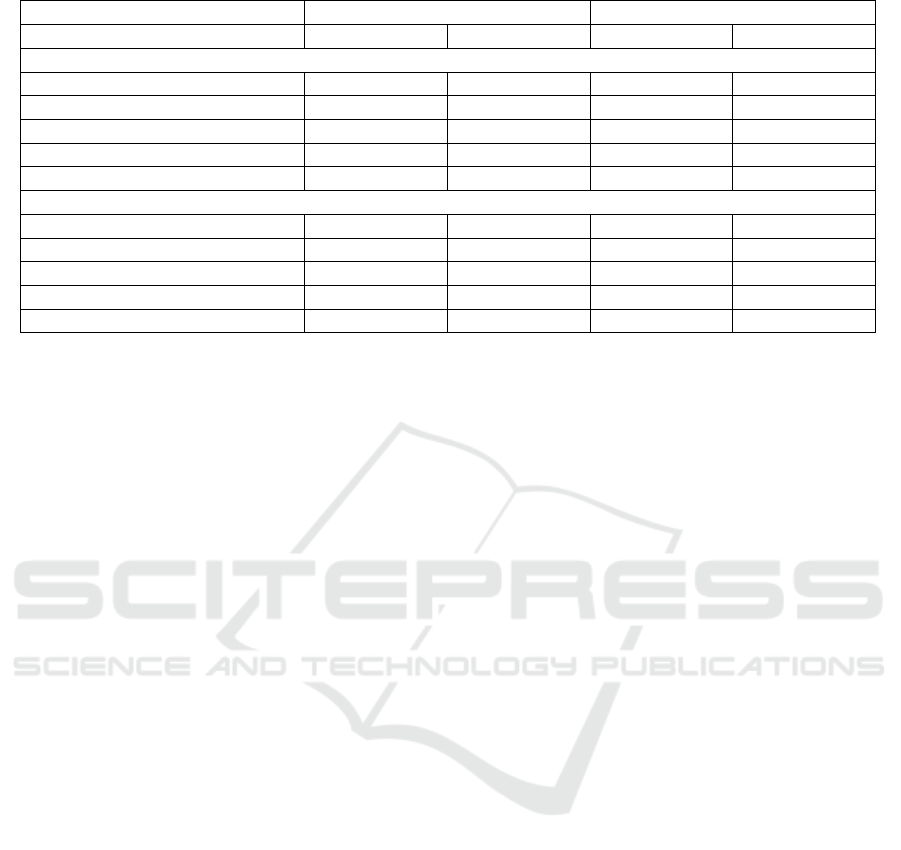
Table 2: Ablation study.

without TTBN with TTBN

Ablation Avg. Val. Acc. Avg. Test Acc. Avg. Val. Acc. Avg. Test Acc.

PACS dataset

Double branch only (A) 96.8 ± 0.6 53.4 ± 2.6 96.4 ± 0.3 67.4 ± 0.8

Detached loss term (B) 97.5 ± 0.1 52.6 ± 2.3 97.3 ± 0.3 68.2 ± 1.3

Secondary prediction branch (C) 98.0 ± 0.1 53.4 ± 2.8 96.9 ± 0.2 70.1 ± 0.4

Single branch (D) 92.8 ± 1.1 46.4 ± 4.9 93.0 ± 0.9 51.2 ± 5.1

Complete method 98.6 ± 0.2 56.1 ± 2.7 96.4 ± 0.3 71.3 ± 0.6

Ofﬁce-Home dataset

Double branch only (A) 82.7 ± 0.4 52.8 ± 0.5 82.6 ± 0.3 53.5 ± 0.4

Detached loss term (B) 83.5 ± 0.7 52.7 ± 0.6 82.3 ± 0.6 54.0 ± 0.6

Secondary prediction branch (C) 81.3 ± 0.4 53.9 ± 0.7 83.8 ± 0.6 54.8 ± 0.5

Single branch (D) 82.6 ± 0.7 53.7 ± 0.4 82.0 ± 0.5 54.3 ± 0.5

Complete method 84.0 ± 0.6 53.4 ± 0.6 83.8 ± 0.5 54.5 ± 0.3

the highest when our approach or ERM is used and

only reaches a result closely similar to ERM or below

in most of the other cases. We hypothesize that the

domain shifts of the PACS datasets are mostly tex-

tures shifts, while they are not for the Ofﬁce-Home

datasets. This would explain why test-time batch nor-

malization yields a large improvement on the PACS

benchmark: the simple use of test-time statistics, that

encode textures (Benz et al., 2021), is enough to sig-

niﬁcantly bridge the domain gap. It would also ex-

plain why the methods reaching the highest results

(Zhang et al., 2022b; Nam et al., 2021; Wang et al.,

2021b) in the usual setting (without test-time batch

normalization) are all style-transfer-based methods.

As our approach is not related to style transfer in

any way, we are able to reach a higher accuracy on

Ofﬁce-Home than other existing works. Regarding

the effect of different training-time methods, we hy-

pothesize that the magnitude of the gain is related to

whether the method is really learning a more diverse

set of patterns or rather only weighting differently pat-

terns that would also be learned naturally. This would

explain why several methods that improve upon ERM

without test-time batch normalization only perform

precisely as well once it is used. Style-transfer-based

methods, for instance, essentially grant a higher im-

portance to shape-based patterns rather than texture-

based patterns but not necessarily learn new patterns.

We also conducted an extensive ablation study

to understand and demonstrate the necessity of our

choices. As a sanity check, we ﬁrst study the α = 0

situation: a single features extractor on which two

classiﬁcation layers are plugged in, trained only

with the cross-entropy on the same batch at each

iteration for both branches (line A in the table 2).

The differences in initialization of the classiﬁers

may have an implicit ensembling effect, as in MIMO

(Havasi et al., 2021), which could lead to a better out-

of-distribution generalization without the need for

the shortcut avoidance loss. This experiment yields a

small increase of performance on both benchmarks,

but it remains far below our approach, whose gain is,

therefore, not coming from an implicit ensembling

mechanism. We also study the effect of detaching

from the computational graph the c

( f (W, ˜x

)) term

(not optimizing the features extractor with respect

to this part of the loss) in the shortcut avoidance

loss (line B), as this could lead to a substantial

improvement in memory consumption, and as the

simultaneous optimization on both terms in not

needed per se to decrease the generalization ability

of the network. This experiment shows a decreased

performance as well. The detachment most likely

only results in a slower learning as the constraint’s

gradient pushes in the reverse direction of the classiﬁ-

cation loss gradient. This behavior is prevented when

the features extractor is optimized with regard to both

terms of the regularization: pushing in the reverse

direction of the classiﬁcation gradient will only slide

the difference in the parameter space but not shorten

the gap. Then, to show that the performance gain

is effectively linked to a mitigation of the shortcut

learning phenomenon, we conduct two experiments.

Firstly, we study the impact of using the secondary

prediction branch at test-time rather than the primary

one (line C). This experiment results in performances

fairly similar to the ﬁrst branch, only lower in

validation. This was to be expected as the secondary

branch is precisely trained so that it generalizes less

on the training domain. Secondly, we study the

effect of applying our shortcut avoidance loss on

an architecture without the added secondary branch

(line D). The shortcut avoidance loss is thus applied

to the original classiﬁer. The results show a dramatic

VISAPP 2023 - 18th International Conference on Computer Vision Theory and Applications

354

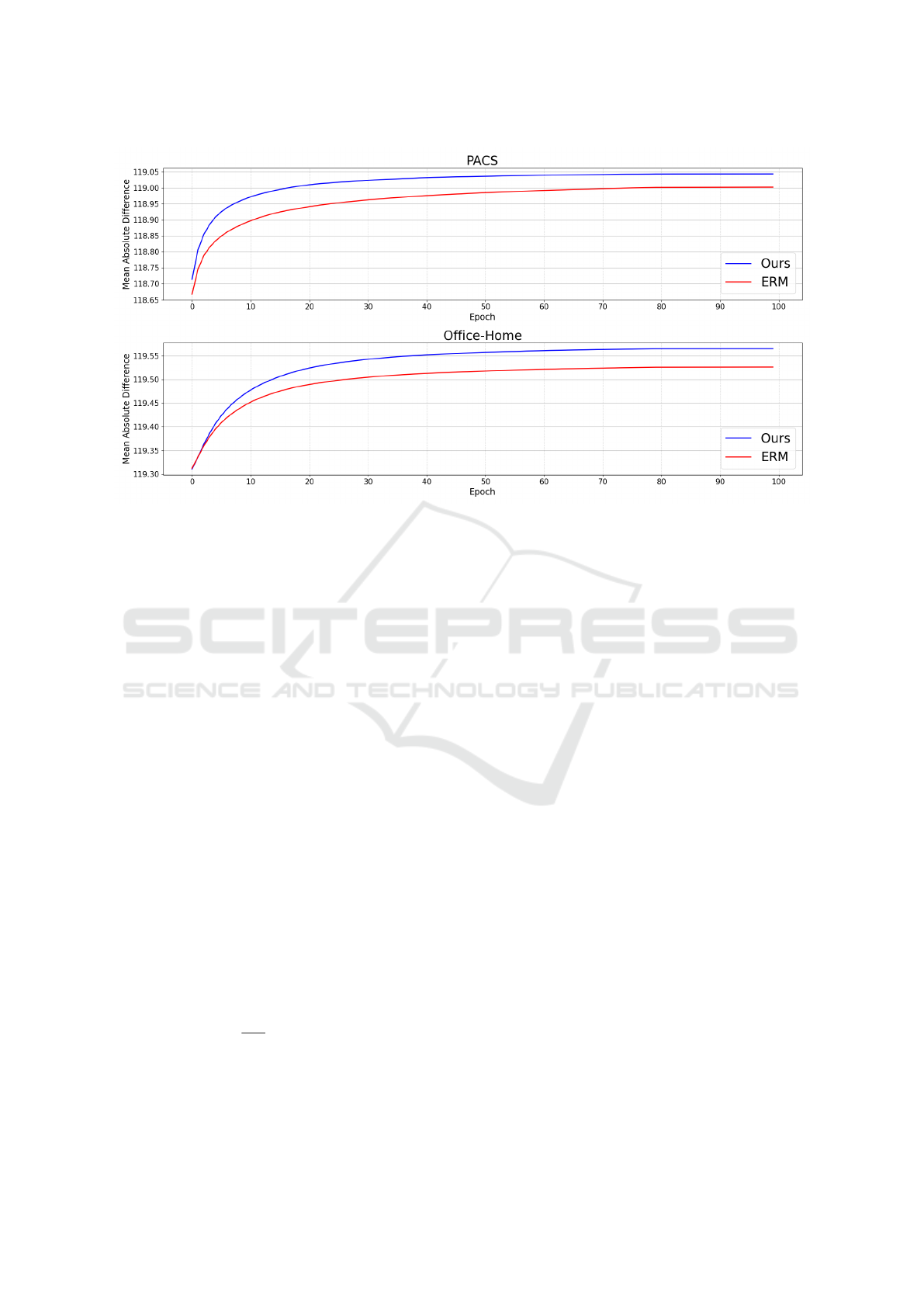
Figure 2: Mean absolute difference for ERM and our approach.

drop in accuracy on the PACS dataset but not on the

Ofﬁce-Home dataset. This difference is most likely

due to the higher diversity in Ofﬁce-Home, which

prevents the original patterns from being ignored.

To further show the effect of our loss, we track

during training a measure of the diversity of the

learned patterns for both our approach and ERM. In-

spired by (Ayinde et al., 2019), we use the mean ab-

solute difference (MAD) between normalized convo-

lutional ﬁlters f (or neurons for fully connected lay-

ers) of a certain layer, computed over all layers L of

size N

and training domains D, for an epoch t, fol-

lowing the equation 1. The results are available in

ﬁgure 2 and show a systematic increase in the diver-

sity of the learned patterns for our approach compared

to ERM, for both benchmarks. Finally, as the tun-

ing of hyper-parameters in the domain generalization

setting is a critical issue, we conduct a broad hyper-

parameters sensitivity analysis, available in the sup-

plementary material in table 3. Our study shows a

relatively low sensitivity and a large match between

hyper-parameters ﬁt for all training-test pairs of PACS

and Ofﬁce-Home.

MAD(t) =

∑

i, j

|| f

t,D,L,i

− f

t,D,L, j

(1)

5 CONCLUSION

In this paper, we investigated the behavior of dif-

ferent single-source methods when used in conjunc-

tion with test-time batch normalization on the PACS

and Ofﬁce-Home benchmarks. We showed that test-

time batch normalization always has a positive, yet

highly variable, inﬂuence and that, most of the time,

the addition of a training-time method is superﬂuous.

We hypothesized that this lack of additional perfor-

mance was linked to the selection behavior of some

algorithms, which still learn the same subset of pat-

terns as the standard training, but weigh them dif-

ferently. We thus proposed a novel approach learn-

ing normally ”hidden” patterns by looking for pre-

dictive patterns that generalize less. We showed that

it yielded state-of-the-art results on both benchmarks

and beneﬁts the most to test-time batch normalization.

Future work will be dedicated to a better understand-

ing of the origin of this test-time batch normalization

variability and to experiments with our method on the

DomainBed (Gulrajani and Lopez-Paz, 2021) bench-

mark.

ACKNOWLEDGEMENTS

This work was in part supported by the 4D Vision

project funded by the Partner University Fund (PUF),

a FACE program, as well as the French Research

Agency, l’Agence Nationale de Recherche (ANR),

Learning Less Generalizable Patterns for Better Test-Time Adaptation

355

through the projects Learn Real (ANR-18-CHR3-

0002-01), Chiron (ANR-20-IADJ-0001-01), Aristo-

tle (ANR-21-FAI1-0009-01), and the joint support of

the French national program of investment of the fu-

ture and the regions through the PSPC FAIR Waste

project.

REFERENCES

Ayinde, B. O., Inanc, T., and Zurada, J. M. (2019). Regu-

larizing deep neural networks by enhancing diversity

in feature extraction. IEEE Transactions on Neural

Networks and Learning Systems.

Beery, S., Van Horn, G., and Perona, P. (2018). Recognition

in terra incognita. In IEEE/CVF European conference

on computer vision.

Benz, P., Zhang, C., Karjauv, A., and Kweon, I. S. (2021).

Revisiting batch normalization for improving corrup-

tion robustness. In IEEE/CVF Winter Conference on

Applications of Computer Vision.

Carlucci, F. M., D’Innocente, A., Bucci, S., Caputo, B., and

Tommasi, T. (2019). Domain generalization by solv-

ing jigsaw puzzles. In IEEE/CVF Conference on Com-

puter Vision and Pattern Recognition.

DeGrave, A. J., Janizek, J. D., and Lee, S.-I. (2021). Ai for

radiographic covid-19 detection selects shortcuts over

signal. Nature Machine Intelligence.

Finn, C., Abbeel, P., and Levine, S. (2017). Model-agnostic

meta-learning for fast adaptation of deep networks. In

International Conference on Machine Learning.

Galanti, T. and Poggio, T. (2022). Sgd noise and implicit

low-rank bias in deep neural networks. arXiv preprint

arXiv:2206.05794.

Geirhos, R., Jacobsen, J.-H., Michaelis, C., Zemel, R.,

Brendel, W., Bethge, M., and Wichmann, F. A. (2020).

Shortcut learning in deep neural networks. Nature

Machine Intelligence.

Gokhale, T., Anirudh, R., Thiagarajan, J. J., Kailkhura, B.,

Baral, C., and Yang, Y. (2022). Improving diversity

with adversarially learned transformations for domain

generalization. arXiv preprint arXiv:2206.07736.

Gulrajani, I. and Lopez-Paz, D. (2021). In search of lost

domain generalization. In International Conference

on Learning Representations.

Havasi, M., Jenatton, R., Fort, S., Liu, J. Z., Snoek, J., Lak-

shminarayanan, B., Dai, A. M., and Tran, D. (2021).

Training independent subnetworks for robust predic-

tion. In International Conference on Learning Repre-

sentations.

He, K., Zhang, X., Ren, S., and Sun, J. (2016). Deep resid-

ual learning for image recognition. In IEEE/CVF Con-

ference on Computer Vision and Pattern Recognition.

Hermann, K., Chen, T., and Kornblith, S. (2020). The ori-

gins and prevalence of texture bias in convolutional

neural networks. Advances in Neural Information

Processing Systems.

Hermann, K. and Lampinen, A. (2020). What shapes

feature representations? exploring datasets, architec-

tures, and training. Advances in Neural Information

Processing Systems.

Hoffman, J., Tzeng, E., Park, T., Zhu, J.-Y., Isola, P.,

Saenko, K., Efros, A., and Darrell, T. (2018). Cy-

cada: Cycle-consistent adversarial domain adaptation.

In International Conference on Machine Learning.

Hu, X., Uzunbas, G., Chen, S., Wang, R., Shah, A., Nevatia,

R., and Lim, S.-N. (2021). Mixnorm: Test-time adap-

tation through online normalization estimation. arXiv

preprint arXiv:2110.11478.

Huang, R., Xu, B., Schuurmans, D., and Szepesv

ari, C.

(2015). Learning with a strong adversary. arXiv

preprint arXiv:1511.03034.

Huang, Z., Wang, H., Xing, E. P., and Huang, D. (2020).

Self-challenging improves cross-domain generaliza-

tion. In IEEE/CVF European Conference on Com-

puter Vision.

Huh, M., Mobahi, H., Zhang, R., Cheung, B., Agrawal, P.,

and Isola, P. (2021). The low-rank simplicity bias in

deep networks. arXiv preprint arXiv:2103.10427.

Jackson, P. T., Abarghouei, A. A., Bonner, S., Breckon,

T. P., and Obara, B. (2019). Style augmentation: data

augmentation via style randomization. In IEEE/CVF

Conference on Computer Vision and Pattern Recogni-

tion Workshops.

Krueger, D., Caballero, E., Jacobsen, J.-H., Zhang, A., Bi-

nas, J., Priol, R. L., and Courville, A. (2020). Out-of-

distribution generalization via risk extrapolation (rex).

arXiv preprint arXiv:2003.00688.

Kurakin, A., Goodfellow, I. J., and Bengio, S. (2016). Ad-

versarial machine learning at scale. In International

Conference on Learning Representations.

Li, D., Yang, Y., Song, Y.-Z., and Hospedales, T. M. (2017).

Deeper, broader and artier domain generalization. In

IEEE/CVF International Conference on Computer Vi-

sion.

Li, D., Yang, Y., Song, Y.-Z., and Hospedales, T. M.

(2018a). Learning to generalize: Meta-learning for

domain generalization. In Thirty-Second AAAI Con-

ference on Artiﬁcial Intelligence.

Li, H., Jialin Pan, S., Wang, S., and Kot, A. C. (2018b).

Domain generalization with adversarial feature learn-

ing. In IEEE/CVF Conference on Computer Vision

and Pattern Recognition.

Moyer, D., Gao, S., Brekelmans, R., Galstyan, A., and

Ver Steeg, G. (2018). Invariant representations with-

out adversarial training. In Advances in Neural Infor-

mation Processing Systems.

Nado, Z., Padhy, S., Sculley, D., D’Amour, A., Lak-

shminarayanan, B., and Snoek, J. (2020). Eval-

uating prediction-time batch normalization for ro-

bustness under covariate shift. arXiv preprint

arXiv:2006.10963.

Nam, H., Lee, H., Park, J., Yoon, W., and Yoo, D. (2021).

Reducing domain gap by reducing style bias. In

IEEE/CVF Conference on Computer Vision and Pat-

tern Recognition.

VISAPP 2023 - 18th International Conference on Computer Vision Theory and Applications

356

Pezeshki, M., Kaba, S.-O., Bengio, Y., Courville, A., Pre-

cup, D., and Lajoie, G. (2020). Gradient starvation: A

learning proclivity in neural networks. arXiv preprint

arXiv:2011.09468.

Schneider, S., Rusak, E., Eck, L., Bringmann, O., Bren-

del, W., and Bethge, M. (2020). Improving robustness

against common corruptions by covariate shift adap-

tation. Advances in Neural Information Processing

Systems.

Shah, H., Tamuly, K., Raghunathan, A., Jain, P., and Ne-

trapalli, P. (2020). The pitfalls of simplicity bias in

neural networks. In Advances in Neural Information

Processing Systems.

Shi, B., Zhang, D., Dai, Q., Zhu, Z., Mu, Y., and Wang, J.

(2020). Informative dropout for robust representation

learning: A shape-bias perspective. In International

Conference on Machine Learning.

Singla, S., Nushi, B., Shah, S., Kamar, E., and Horvitz, E.

(2021). Understanding failures of deep networks via

robust feature extraction. In IEEE/CVF Conference on

Computer Vision and Pattern Recognition.

Srivastava, N., Hinton, G., Krizhevsky, A., Sutskever, I.,

and Salakhutdinov, R. (2014). Dropout: A simple way

to prevent neural networks from overﬁtting. Journal

of Machine Learning Research.

Venkateswara, H., Eusebio, J., Chakraborty, S., and Pan-

chanathan, S. (2017). Deep hashing network for un-

supervised domain adaptation. In IEEE/CVF Confer-

ence on Computer Vision and Pattern Recognition.

Volpi, R., Namkoong, H., Sener, O., Duchi, J. C., Murino,

V., and Savarese, S. (2018). Generalizing to unseen

domains via adversarial data augmentation. In Ad-

vances in Neural Information Processing Systems.

Wang, D., Shelhamer, E., Liu, S., Olshausen, B., and Dar-

rell, T. (2021a). Tent: Fully test-time adaptation by

entropy minimization. In International Conference on

Learning Representations.

Wang, Z., Luo, Y., Qiu, R., Huang, Z., and Baktashmot-

lagh, M. (2021b). Learning to diversify for single do-

main generalization. In IEEE/CVF International Con-

ference on Computer Vision.

Xu, Z., Liu, D., Yang, J., Raffel, C., and Niethammer, M.

(2021). Robust and generalizable visual representa-

tion learning via random convolutions. In Interna-

tional Conference on Learning Representations.

Yang, T., Zhou, S., Wang, Y., Lu, Y., and Zheng, N.

(2022). Test-time batch normalization. arXiv preprint

arXiv:2205.10210.

You, F., Li, J., and Zhao, Z. (2021). Test-time batch statis-

tics calibration for covariate shift. arXiv preprint

arXiv:2110.04065.

Zhang, M. M., Levine, S., and Finn, C. (2021). Memo: Test

time robustness via adaptation and augmentation. In

NeurIPS 2021 Workshop on Distribution Shifts: Con-

necting Methods and Applications.

Zhang, X., Zhou, L., Xu, R., Cui, P., Shen, Z., and

Liu, H. (2022a). Nico++: Towards better bench-

marking for domain generalization. arXiv preprint

arXiv:2204.08040.

Zhang, Y., Li, M., Li, R., Jia, K., and Zhang, L. (2022b).

Exact feature distribution matching for arbitrary style

transfer and domain generalization. In IEEE/CVF

Conference on Computer Vision and Pattern Recog-

nition.

Zhao, L., Liu, T., Peng, X., and Metaxas, D. (2020).

Maximum-entropy adversarial data augmentation for

improved generalization and robustness. Advances in

Neural Information Processing Systems.

SUPPLEMENTARY MATERIAL

Results Details

The results were obtained as follows:

• For the 12 distinct pairs of training and test do-

mains, we calculate the average and the standard

deviation of the validation and test accuracies over

3 runs with different random seeds (because the

effect of the network’s initialization on the test ac-

curacy is greater than usual in a test-time domain

shift situation).

• The reported numbers are the non-weighted mean

over all distinct pairs of the average accuracies per

training-test pair previously computed ± the mean

over all distinct pairs of the pairwise standard de-

viation (as we are interested in the randomness of

the initialization rather than the variation of accu-

racies between training-test pairs).

Hyper-parameters Details

Data: for all the methods and benchmarks, we use

the data augmentation described in (Huang et al.,

2020) (random resized crops, color jitter, random

horizontal ﬂips, random grayscale). For a particular

domain used in training, 90% of the dataset is used

for training and the remaining 10% for validation.

The test set is obtained using another domain dataset

entirely.

Common Hyper-parameters: experiments were

conducted with a ResNet18 (He et al., 2016) trained

for 100 epochs, with the stochastic gradient descent,

a learning rate of 1e − 3, a batch size of 64, a weight

decay of 1e − 5, and a Nesterov momentum of 0.9.

After 80 epochs, the learning rate is divided by 10.

The exponential average momentum used in the

batch normalization layers at test-time is set to 0.1.

L2GP (ours): the gradient ascent learning rate lr

set to 1.0 and the α weight for the shortcut avoidance

loss to 1.0 as well, for all the experiments, that is,

Learning Less Generalizable Patterns for Better Test-Time Adaptation

357

Table 3: Broad hyper-parameters sensitivity analysis.

Avg. test Acc. on PACS - Avg. test Acc. on Ofﬁce-Home

↓ / α → 10

−3

−2

0.1 1.0 10.0 100.0

−3

66.9 - 53.7 66.8 - 53.1 67.7 - 53.2 67.0 - 53.5 67.4 - 53.2 68.5 - 53.7

−2

67.8 - 53.2 67.8 - 53.1 67.6 - 53.3 67.7 - 52.4 68.6 - 53.9 70.6 - 53.2

0.1 67.8 - 53.0 67.5 - 53.2 67.4 - 53.3 69.5 - 53.8 71.3 - 54.7 69.2 - 51.9

1.0 67.1 - 53.3 68.0 - 53.4 69.0 - 53.8 71.3 - 54.4 70.3 - 52.6 20.1 - 49.9

10.0 67.8 - 52.9 67.2 - 53.4 67.4 - 53.3 66.0 - 53.9 54.4 - 51.9 15.0 - 5.2

100.0 66.2 - 53.2 67.9 - 53.4 67.4 - 53.4 67.8 - 53.3 60.5 - 53.2 14.5 - 2.0

for all the training-test pairs on both the PACS and

the Ofﬁce-Home datasets. These hyper-parameters

were ﬁrst set arbitrarily to plausible values and then

conﬁrmed to be effective on the PACS benchmark

by looking at target performance. They were ﬁ-

nally reused as is on the Ofﬁce-Home benchmark.

This hyper-parameters selection strategy may seem

sub-optimal but is, in fact, more and more used in

domain generalization problems (Gokhale et al.,

2022; Xu et al., 2021): a method requiring a new and

careful hyper-parameters setting for each new dataset

encountered is impractical, even more so when the

target data distribution is unknown and cannot thus

be used to help the setting.

Comparison baselines speciﬁcs hyper-parameters are

detailed below. For the experiments on the PACS

datasets, on which most of the baselines were tested,

we use the same hyper-parameters as in the original

works. For the Ofﬁce-Home datasets, we used

the hyper-parameters of the multi-source setting if

available. If the methods did not have quantitative

hyper-parameters, such as EFDM (Zhang et al.,

2022b) with the choice of mixing-layers depths, we

used the ones proposed for the PACS experiments for

the ones on Ofﬁce-Home. Likewise, if no rigorous

hyper-parameters setting strategy was detailed in the

original work, we used the PACS hyper-parameters

for experiments on Ofﬁce-Home. Finally, for the

Spectral Decoupling work that was never evaluated

on neither PACS nor Ofﬁce-Home, we conducted

a simple hyper-parameters search using a single

training-test domains pair, and transferred them as is

to the other pairs with the same training domain.

RSC: the percentage of channels (or spatial cross-

channel locations) to be dropped is initialized at

30% and is increased every 10 epochs linearly to

reach 90% for the last ten. Spatial cross-channel

locations dropout and channel all-locations dropout

are applied in a mutually exclusive way with the

same probability. All samples in a batch are subject

to dropout.

InfoDrop: half the layers are subjected to the

info-dropout. The dropout rate is set to 1.5, the

temperature to 0.1, the bandwidth to 1.0, and the

radius to 3.

ADA: the number of adversarial gradient ascent steps

is set to 25, and the learning rate for the adversarial

gradient ascent steps is set to 50. The γ and η factors

are respectively set to 10.0 and 50.0. Adversarial

images are added to the training set every 10 epoch.

ME-ADA: The same hyper-parameters as the ones

above are used.

EFDM: the EFDMix layers are inserted after the ﬁrst

3 residual blocks in the ResNet architecture.

SagNet: The randomization stage and the adversarial

weight of SagNets are ﬁxed to 3 and 0.1 for all

experiments, as in the original work. A gradient

clipping to 0.1 is applied to the adversarial loss.

L.t.D: α

and α

weights for the additional losses

were set to 1.0, β to 0.1, for all experiments.

Spectral Decoupling: the weight of the spectral de-

coupling constraint (an L2-norm on the network’s out-

put) is set to 0.001 for experiments on Ofﬁce-Home

Experiments, and to 0.01 for experiments on PACS.

VISAPP 2023 - 18th International Conference on Computer Vision Theory and Applications

358