There is More than Mean and Variance on Waiting

Dominik Berbig

Pforzheim University, Business School, BW/Purchasing and Logistics, Tiefenbronner Str. 65, 75175 Pforzheim, Germany

Keywords: Queuing Theory, Discrete-Time Modelling, Waiting Times, Skewness, Kurtosis.

Abstract: Processes in material flow systems, which can be regarded as queuing systems, are discrete in time.

Nevertheless, the main research work considering queuing theory focuses on time-continuous modelling.

However, for G/G/m-queues in continuous time, analysis relevant parameters can only be estimated and not

exactly calculated anymore. These approximations are based on the first two central moments of the inter-

arrival and service time distribution only and can be arbitrarily wrong. Considering discrete-time approach,

the parameters can be calculated exactly. This means that also other central moments of according

distributions may have an effect that is not to be neglected. Thus, in this paper we investigate the effect of

skewness and kurtosis of service time distributions on the expected waiting times for queuing customers. In

order to do so, we modelled queuing systems in a discrete-time manner and calculated resulting waiting times

for distributions having the same mean and variance. In continuous time approximation, the result is always

the same. Exact calculations following a discrete-time approach show differences of more than 15 %.

Afterwards, we investigated on the effect the skewness and kurtosis of the according distributions have. First

findings and need for further research are presented in this position paper.

1 INTRODUCTION

Time (perhaps not physically speaking) is a

continuous flow. Thus, the normal assumption when

modelling material flow systems by applying queuing

theory is to consider processes to happen in

continuous time. For the M/M/1- or M/G/1-queue this

works perfectly well and relevant parameters such as

waiting or sojourn times can be calculated exactly.

However, as soon as the Markovian property isn´t

valid for the arrival process anymore, i.e. inter-arrival

times are generally distributed, these parameters can´t

be calculated exactly anymore, compare (Furmans,

1999). They can only be estimated approximately.

Common to all these approximations is that they are

based on the mean as well as the standard deviation

of the arrival process exclusively. Consequently, the

result of such an approximation is always the same

even for different distributions as long as their mean

and standard deviation are identical. Besides,

different approximations lead to different results. And

they can – even worse – be arbitrarily wrong,

according to (Furmans, 1999). However, processes in

material flow systems can be seen as time discrete,

https://orcid.org/0009-0003-2641-1158

compare (Schleyer, 2007): Even if the time remains

continuous, certain events do only take place at

certain points in time: Let´s take the arrival process of

trucks at a warehouse for example. Here, it is not

relevant if trucks arrive in time considering

milliseconds or even seconds. It is enough to measure

it in minutes or with regards to even coarser time

windows of e.g. 30 mins each. Or take milk runs for

material supply at production areas. Also here, it´s

minutes that count in general. Even for production

itself, cycle times are measured in seconds. Thus,

discrete-time modelling can be used. When applying

discrete-time modelling, all relevant parameters

(waiting time, sojourn time, number of customers

within the system…) can be calculated exactly as now

the complete distributions for the arrival as well as the

service process are known – at least in an ε-

environment as denoted in (Schleyer, 2007). No

approximations are needed, different distributions

lead to different results. An example for the beneficial

applying of discrete-time queuing theory for

analysing a manufacturing line can be found in

(Furmans, Berbig and Fleischmann, 2009).

Consequently, we apply discrete-time modelling

Berbig, D.

There is More than Mean and Variance on Waiting.

DOI: 10.5220/0011947400003546

In Proceedings of the 13th International Conference on Simulation and Modeling Methodologies, Technologies and Applications (SIMULTECH 2023), pages 171-177

ISBN: 978-989-758-668-2; ISSN: 2184-2841

 2023 by SCITEPRESS – Science and Technology Publications, Lda. Under CC license (CC BY-NC-ND 4.0)

171

within this paper. The target of this work is to identify

if the third (skewness) and fourth (kurtosis)

centralized moment of the inter-arrival time

distribution have an effect on customer´s waiting

times – and if so, which effect could this be. Reason

for this is that approximations in continuous time can

be calculated rather easily, however exact

calculations with discrete-time modelling is more

complex and cannot be done as easily.

2 G/G/1-QUEUING SYSTEMS IN

CONTINUOUS AND DISCRETE

TIME

In the following, we use Kendall´s Notation A/B/m

where A indicates the inter-arrival time distribution,

B the service time distribution and m the number of

servers, as depicted e.g. in (Schleyer, 2007). G

indicates that the distribution is a general one, i.e. the

Markovian property is not given, the underlying

distribution is not an exponential one.

We consider G/G/1-queues where inter-arrival

and service times are uid. For these, amongst others

(Marchal, 1976) has derived an approximation

formula (1) to calculate the customer´s waiting times

in the queuing system. It can be denoted as:

𝐸



𝑡



























∙













(1)

Where

 E(t

) = expected waiting time

 𝑐





= variability of service process

 𝜌 = utilization of service station

 𝑉𝑎𝑟𝑇



 = variance of inter-arrival time

distribution

 𝑉𝑎𝑟𝑇



 = variance of service time

distribution

 𝜆 = arrival rate of customers at service

station

Besides, several other approximations have been

developed, e.g. by (Krämer-Langenbach-Belz, 1977)

or (Buzacott and Shantikumar, 1993). All these

follow the same basic principle as they are based on

the description of stochastic processes by the first two

moments only. Everything else is neglected. Thus,

they are more or less precise, any size of relative

relative errors can occur (Furmans, 1999). But each

of these approximations will always lead to the same

result even for totally different distributions as long

as their mean and variance are the same. (Schleyer

and Furmans, 2007), (Huber, 2011) and (Matzka,

2011) confirm the above-mentioned findings as well.

In contrast to this, (Grassmann and Jain, 1989)

have shown an exact approach (at least within an ε-

neighbourhood) for determining waiting times by

considering a discrete-time G/G/1-queue. However,

this algorithm is more complex in application. We use

these approximations as well as the algorithm for

comparison as the starting point for further analysis.

Table (acc. Schleyer, 2007) shows the according

results: An arbitrary inter-arrival time distribution (a)

and five different service time distributions (b

), all of

these having the same mean value and variance, have

been taken. With these, the expected waiting times for

customers arriving at the queueing system are

calculated in time-continuous domain, always

following the three above mentioned approximations.

As expected, each approximation leads to the same

waiting times for all five cases while each

approximation leads to different expected values. The

relative difference between the smallest and the

biggest result is 13.17 % taking the lowest result as

basis. Afterwards, the exact algorithm proposed by

Grassmann and Jain applying discrete-time

modelling has been implemented to calculate the

exact expected waiting times for all five cases (b

Here the results differ due to the different service time

distributions. They have a difference of nearly 9 %

taking the lowest result as basis again. Finally, the

maximum absolute and relative deviations between

each approximation and the exact algorithm result

have been calculated. The difference in this case is

between 7.73 % and 10.90 %, always based on the

result calculated according to (Grassmann and Jain,

1989). Those numbers show that there is a significant

difference that may not be neglected. Consequently,

the question on the effect of further central moments

of the distributions arises. Thus, we investigate on the

effect of the skewness (third central moment) and the

kurtosis (fourth central moment) in our work.

3 DETERMINATION OF

DISTRIBUTIONS

To investigate these effects further, we first derive

additional discrete distributions that all have the same

mean and variance. This means, the following

conditions have to be fulfilled where α and β are

values that can be arbitrarily chosen:

𝑃



𝑋𝑥





1





(2)

SIMULTECH 2023 - 13th International Conference on Simulation and Modeling Methodologies, Technologies and Applications

172

Table 1: Comparison for G/G/1-queue in time continuous and discrete-time consideration (acc. Schleyer, 2007).

𝐸



𝑋



 𝜇𝑥



∙𝑃



𝑋 𝑥





𝛼





(3)

𝑉𝑎𝑟



𝑋



𝜎



 𝑥²



∙𝑃



𝑋𝑥





𝜇²𝛽





(4)

For identifying distributions that fulfil equations

(2) – (4), we implemented a small Java program that

follows the logic shown in Figure 1:

Figure 1: Program logic for distribution determination.

This program only requires two arbitrary numbers

as input variables: the desired mean value as well as

the desired variance. The result of the algorithm are

different discrete distributions which do all fulfil

equations (2) – (4). Consequently, only the first two

centralized moments of each distribution are

predetermined and known. Further centralized

moments, like skewness and kurtosis, are just a

consequence. Even if the program is quite simple, it

is working effectively. All the user has to do is to wait

for results. Using it accordingly, we were able to

identify way more than 150 different distributions

fulfilling restrictions (2) – (4), also applying different

values for α and β. These distributions can serve for

both – as distributions for the inter-arrival times or for

the service times. It should only be noted that for each

selected combination of service and inter-arrival

times, the mean value of the inter-arrival time has to

be greater than the mean value of the service time. In

these cases, the utilization of the queueing system is

less than 1 which means that the queuing system is in

balance. Having this as the basis, we were able to

perform according analyses.

i a(i)

(i)

(i) b

(i)

0 0.000 0.000 0.000 0.000 0.000 0.000

1 0.070 0.000 0.324 0.074 0.050 0.206

2 0.080 0.350 0.000 0.149 0.033 0.144

3 0.110 0.175 0.000 0.315 0.660 0.104

4 0.130 0.150 0.000 0.250 0.024 0.000

5 0.150 0.115 0.475 0.000 0.043 0.175

6 0.140 0.100 0.201 0.000 0.011 0.371

7 0.110 0.040 - 0.111 0.000

8 0.090 0.025 - 0.101 0.179 --

9 0.070 0.025 - - - -

10 0.040 0.02 - - - -

11 0.010 - - - - -

Mean value 5.300 3.905 3.905 3.905 3.905 3.905

Squared coefficient of variation 0.220 0.275 0.275 0.275 0.275 0.275

Utilization 0.737 0.737 0.737 0.737 0.737

Marchal (cont.) E(t

) 2.239 2.239 2.239 2.239 2.239

Krämer-Langenbach-Belz (cont.) E(t

) 2.019 2.019 2.019 2.019 2.019

Buzacott and Shantikumar (cont.) E(t

) 2.285 2.285 2.285 2.285 2.285

Grassmann & Jain (dis.) E(t

) 2.243 2.079 2.230 2.266 2.121

max

(absolute) E(t

) 0.224 0.206 0.211 0.247 0.164

max

(relative) E(t

) 9.99 % 9.91 % 9.46 % 10.90 % 7.73 %

There is More than Mean and Variance on Waiting

173

4 FIRST FINDINGS

For further examination, we used the G/G/1-Batch-

Analyser and the DTQNA, both tools resulting from

research work of the IFL at the KIT. With these tools,

it is possible to calculate e.g. waiting times in

queueing systems applying discrete-time approaches.

One of the main calculation basics of these is the

above-mentioned approach proposed by Grassmann

and Jain. Thus, these tools are ideally suited as basis

for our research. The only input needed are the inter-

arrival time distribution A

and the service time

distributions B

. B

represents a group of distributions

that all have the same mean and variance. A

can be

taken out of the following four different inter-arrival

time distributions:

: (0; 0.07; 0.08; 0.11; 0.13; 0.15; 0.14; 0.11;

0.09; 0.07; 0.04; 0.01)

; µ = 5.3, σ² = 6.19

: (0; 0.2; 0.3; 0.15; 0.05; 0.025; 0; 0; 0; 0; 0;

0.025; 0.1; 0.125; 0.025)

; µ = 5.025, σ² =

22.37

: (0; 0.125; 0.125; 0.125; 0.125; 0.125; 0.125;

0.125; 0.125)

; µ = 4.5, σ² = 5.25

. (0; 0; 0.542; 0.026; 0; 0; 0; 0; 0; 0.247; 0.146;

0.039)

; µ = 5.274, σ² = 13.913

As service time distributions, we took several

different ones resulting out of our simple Java

program. In our first experiment, we used A

and 10

different service time distributions of the type B

where μ = 2 and σ² = 0.92. We calculated E(t

) for all

10 cases. Afterwards, we sorted the 10 service time

distributions according to their corresponding

skewness in an ascending order and drew a diagram

for E(t

) in relation to the skewness of the service

time distributions as illustrated in Figure 2. This

shows a monotonous increase of the waiting time

over the skewness. R² is 99.25 % and thus nearly

maximum.

Figure 2: E(t

) with A

and B

over skewness of B

Afterwards, we analogously considered the effect

of the kurtosis on E(t

). This result is depicted in

Figure 3.

Figure 3: E(t

) with A

and B

over kurtosis of B

Here, too, a monotonous increase can be seen,

even if R² is slightly lower but with still 94.23 %

significantly high. Thus, it seems as if there is a link

between the skewness and the expected waiting time

as well as the kurtosis and E(t

): The bigger these

central moments are, the longer is the waiting time for

customers arriving at the service station. This effect

has to be evaluated closer.

5 CONSIDERATION OF

FURTHER DISTRIBUTIONS

Having seen these behaviours, we changed our

service time distributions to the set B

which contains

26 distributions where μ = 3.32 and σ² = 4.745. We

acted as before, i.e. we calculated the expected

waiting times for customers whose inter-arrival times

are distributed with A

while the service time at the

G/G/1-queuing system is always one out of B

. Figure

4 shows the according results.

Figure 4: E(t

) with A

and B

over skewness of B

SIMULTECH 2023 - 13th International Conference on Simulation and Modeling Methodologies, Technologies and Applications

174

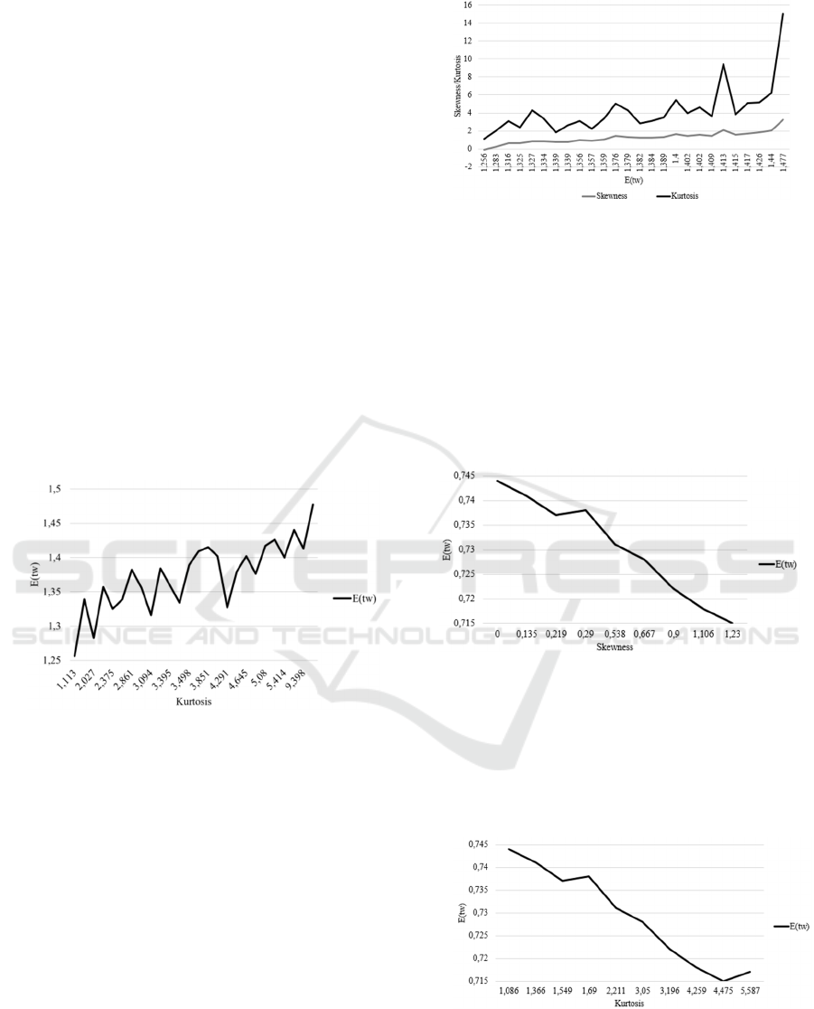
Interestingly, we can see two effects:

 The overall effect of the skewness still

confirms the first findings: A higher skewness

means higher waiting times. R² of 91.60 % is

still significant.

 However, the trend is not a monotone one

anymore. There are cases when a (slightly)

increased skewness leads to a (slightly)

decreased waiting time.

Thus, some questions arise:

 What is the reason for this behaviour?

 Can we see the same behaviour when

considering the kurtosis?

 Which effects do different A

have?

Let´s start with the last two questions and

postpone the first. Considering the kurtosis, the same

two effects confirm: Overall, an increased kurtosis

leads to an increased waiting time. But the

development seems even more “erratic” as depicted

in Figure 5 and thus an R² of only 51.90 %. Here, a

linear relationship cannot be assumed anymore:

Figure 5: E(t

) with A

and B

over kurtosis of B

In order to be able to get some hints regarding this

behaviour, we rearranged the data and sorted E(t

) in

an ascending order and had a look on how the

skewness and the kurtosis develop. Here, we can see

an interesting result: Whenever the skewness

increases from one waiting time to another, the

kurtosis does so as well. However, the kurtosis has

way higher fluctuations than the skewness as Figure

6 shows.

Figure 6: Skewness and kurtosis of B

over E(t

Here, R² is 79,04 % between the skewness and

kurtosis indicating that there could be a connection

between the two moments.

In order to analyse the third question, we did the

same analysis for B

and B

in combination with A

Considering B

at first, the result is shown in Figure

7. Interestingly, there is still a monotonic relationship

between E(t

) and the skewness. R² is even 99.42 %.

However, the relationship is now opposite: An

increased skewness leads to a reduced waiting time.

Figure 7: E(t

) with A

and B

over skewness of B

The same is valid considering the effect of the

kurtosis on the expected waiting time. Even if R² with

90.69 % is slightly smaller, it is still rather high.

However, the trend is not that smooth than it is when

considering the skewness. This can be seen in Figure

Figure 8: E(t

) with A

and B

over Kurtosis of B

What is now the result when considering B

Here, the same change in behaviour is seen as for B

as can be seen in Figure 9: The overall trend does now

There is More than Mean and Variance on Waiting

175

show a reduction of E(t

) when skewness and kurtosis

increase. Here as well, the according R² is now

smaller than when considering A

, namely 42.22 % or

5.50 % indicating that a linear connection cannot be

assumed anymore.

Figure 9: E(t

) with A

and B

over skewness of B

Having seen these results, we calculated the

results for applying A

and B

, A

and B

, A

and B

or A

and B

respectively as input distributions.

Applying A

leads to the same behaviours like A

, A

doesn’t nearly show any systematic behaviour

anymore. Why can this be the case? Considering the

squared coefficients of variation (SCV) of the four

inter-arrival time distributions, we get the following

results:

Table 2: SCV for different A

Inter-arrival time

distribution

Squared coefficient of

variation

0.220

0.886

0.259

0.500

Considering these results, it could be that a

squared coefficient of variation...

 which is below 0.5 indicates a positive

 which is higher than 0.5 leads to a negative

 which is around 0.5 leads to no

correlation between the expected waiting time for

arriving customers and the skewness or kurtosis of the

service time distribution. The same seems valid when

considering the skewness of these four distributions

which is:

Table 3: Skewness for different A

Inter-arrival time

distribution

Skewness

0.120

0.927

0.000

0.312

To further explore the above-mentioned findings

and ideas, we conducted another experiment in which

we chose an arbitrary inter-arrival time distribution

: (0; 0; 0.419; 0.224; 0.143; 0.002; 0.04; 0.119;

0; 0.039; 0; 0.014)

; µ = 3.67, σ² = 4.69

For A

, the squared coefficient of variation is

0.348, the skewness is 1.411, the kurtosis is 1.146.

Again, we took the set B

for service time

distributions and calculated the according expected

waiting times for arriving customers at the queuing

system. Afterwards, we arranged them again over the

skewness and kurtosis of B

. The result can be seen in

the following Figure 10:

Figure 10: E(t

) with A

and B

over skewness of B

In this case, increasing skewness – at least

considering the trend – leads to a shorter waiting time.

The same behaviour can be observed when

considering the kurtosis of B

. However, since in this

case the SCV of A

is smaller than 0.5, this behaviour

contradicts the above assumption. The skewness of

, however, is much larger than 0.5. This could

indicate that SCV and skewness may not be

considered individually, but in combination:

 SCV and skewness below 0.5 indicate a

positive

 SCV below 0.5, but skewness > 1 indicate a

negative

correlation between the expected waiting time for

arriving customers. However, these are just first

assumptions needing further and more detailed

research.

6 CONCLUSION AND OUTLOOK

ON FURTHER RESEARCH

Even if we were not able to identify a clear correlation

between the skewness or kurtosis of the service time

SIMULTECH 2023 - 13th International Conference on Simulation and Modeling Methodologies, Technologies and Applications

176

distribution and the expected waiting times, we

generated some important findings and were able to

show the need for further research:

1. Considering the mean value and the variance

only for inter-arrival and service time

distributions is not sufficient. There can be

differences in the resulting expected waiting

times from more than 15 % (e.g. considering

case A

and B

2. Skewness and kurtosis seem to have an

influence on E(t

3. Skewness and kurtosis show similar

behaviours regarding the development of E(t

4. There might be a correlation between the

squared coefficient of variation and the

skewness of the inter-arrival time distribution

and the effect the skewness or kurtosis have on

the expected waiting time for arriving

customers.

5. Fluctuations within the effect of kurtosis on

E(t

) could be higher due to the underlying

statistics as skewness incorporates the

difference between the observation and the

mean to the power of three, i.e. negative results

can be possible, whereas the kurtosis

incorporates the same difference but to the

power of four, i.e. there can be only values ≥ 0

and the effect of the difference can be higher

(in case it is > 1) than regarding the skewness

or lower (otherwise).

These findings serve as basis for further research

we are currently conducting.

REFERENCES

Buzacott. J.A.. Shantikumar, J.G. (1993). Stochastic

Models of Manufacturing Systems. Prentice Hall.

Englewood Cliffs

Furmans. K. (1999). Bedientheoretische Methoden

als Hilfsmittel der Materialflußplanung.

Habilitationsschrift. Institut für Fördertechnik und

Logistiksysteme. Universität Karlsruhe (TH)

(nowadays KIT)

Furmans. K.. Berbig. D.. Fleischmann. T. (2009).

Evaluating the potential of new material handling

equipment with stochastic finite elements analysis.

Proceedings of the Seventh International Conference on

"Stochastic Models of Manufacturing and Service

Operations", June 7 - 12, 2009, Ostuni, Italy, 142–150,

Aracne, Roma

Grassmann. W.K.. Jain. J.L. (1989). Numerical Solutions of

the Waiting Time Distribution and Idle Time

Distribution of the Arithmetic GI/G/1Queue.

Operations Research, 37

Huber. C. (2011). Throughput Analysis of Manual Order

Picking Systems with Congestion Consideration.

Dissertation. Institut für Fördertechnik und

Logistiksysteme. Karlsruher Institut für Technologie

(KIT).

Krämer. W.. Langenbach-Belz. M. (1977). Approximate

Formula for General Single Server Systems with Single

and Batch Arrivals. Forschungsbericht. Institut für

Nachrichtenvermittlung und Datenverarbeitung.

Universität Stuttgart.

Matzka. J. M. (2011). Discrete Time Analysis of Multi-

Server Queueing Systems in Material Handling and

Service. Dissertation. Institut für Fördertechnik und

Logistiksysteme. Karlsruher Institut für Technologie

(KIT).

Schleyer. M. (2007). Discrete Time Analysis of Batch

Processes in Material Flow Systems. Dissertation.

Institut für Fördertechnik und Logistiksysteme.

Universität Karlsruhe (TH) (nowadays KIT)

Schleyer. M.. Furmans. K. (2007). An analytical method for

the calculation of the waiting time distribution of a

discrete time G/G/1-queueing system with batch

arrivals. OR Spectrum 29(4), p. 745–763.

There is More than Mean and Variance on Waiting

177