Multi-Scale Surface Normal Estimation from Depth Maps

Diclehan Ulucan, Oguzhan Ulucan and Marc Ebner

Institut für Mathematik und Informatik, Universität Greifswald,

Walther-Rathenau-Straße 47, 17489 Greifswald, Germany

Keywords:

Intrinsic Image Decomposition, Surface Normal Estimation, Depth Map, Scale-Space.

Abstract:

Surface normal vectors are important local descriptors of images, which are utilized in many applications in

the ﬁeld of computer vision and computer graphics. Hence, estimating the surface normals from structured

range sensor data is an important step for many image processing pipelines. Thereupon, we present a simple yet

eﬀective, learning-free surface normal estimation strategy for both complete and incomplete depth maps. The

proposed method takes advantage of scale-space. While the ﬁnest scale is used for the initial estimations, the

missing surface normals, which cannot be estimated properly are ﬁlled from the coarser scales of the pyramid.

The same procedure is applied for incomplete depth maps with a slight modiﬁcation, where we guide the

algorithm using the gradient information obtained from the shading image of the scene, which has a geometric

relationship with the surface normals. In order to test our method for the incomplete depth maps scenario, we

augmented the MIT-Berkeley Intrinsic Images dataset by creating two diﬀerent sets, namely, easy and hard.

According to the experiments, the proposed algorithm achieves competitive results on datasets containing both

single objects and realistic scenes.

1 INTRODUCTION

Surface normal vectors are local descriptors that can

help us to obtain the shape of an object, light di-

rection, and curvature (Ebner, 2007). Many studies

make use of surface normals as auxiliary informa-

tion in computer vision applications such as 3D object

recognition, surface reconstruction, and depth com-

pletion (Harms et al., 2014; Zhang and Funkhouser,

2018; Fan et al., 2021). Since surface normals are uti-

lized in several pipelines, their eﬃcient estimation is

of critical importance.

Surface normals can be extracted from depth

maps/disparity images and 3D point clouds (Mitra and

Nguyen, 2003; Zhang and Funkhouser, 2018). Point

clouds are usually unorganized and distorted by noise,

which causes the requirement of computationally ex-

pensive procedures and complicates the extraction of

features (Awwad et al., 2010; Fan et al., 2021). Thus,

depth maps and disparity images have gained attention

for the task of surface normal estimation, since they

contain structured sensor data. While the close geo-

metric relationship between depth maps and surface

normals is a very useful feature, possible missing in-

formation in depth maps is a challenge, which should

be considered during algorithm design.

Over the years, several surface normal estima-

tion methods have been proposed, which utilize var-

ious approaches (Klasing et al., 2009; Zeng et al.,

2019). For instance, several averaging-based algo-

rithms, such as the area-weighted and angle-weighted

methods, have been introduced, which take advantage

of the local neighbourhood to compute the surface

normals (Klasing et al., 2009). Also, other statistics-

and optimization-based techniques have been pro-

posed to estimate the surface normals. The SIRFS al-

gorithm aims at recovering the reﬂectance, shading,

illumination, surface normals, depth, and shape from

a single masked image (Barron and Malik, 2014).

SIRFS relies on priors and formulates an optimization

problem to recover the intrinsic images. The 3F2N

method applies three ﬁlters namely, a horizontal and

a vertical gradient ﬁlter, and a mean/median ﬁlter, to

structured range sensor data to estimate the surface

normals (Fan et al., 2021). 3F2N utilizes the camera

focal lengths and image principal point as priors.

While traditional methods are still widely used

and new statistical techniques are introduced, with the

improvements in deep learning, convolutional neural

networks-based algorithms have also been developed

for surface normal estimation purposes. However, in

several studies it is discussed that deep learning tech-

Ulucan, D., Ulucan, O. and Ebner, M.

Multi-Scale Surface Normal Estimation from Depth Maps.

DOI: 10.5220/0011968300003497

In Proceedings of the 3rd International Conference on Image Processing and Vision Engineering (IMPROVE 2023), pages 47-56

ISBN: 978-989-758-642-2; ISSN: 2795-4943

 2023 by SCITEPRESS – Science and Technology Publications, Lda. Under CC license (CC BY-NC-ND 4.0)

niques require a high amount of unbiased data to out-

put accurate results and to ﬁnd the optimal parame-

ters for the network (Fan et al., 2021; Ulucan et al.,

2022b; Ulucan et al., 2022c). In the ﬁeld of surface

normal estimation the most commonly used datasets

are collected via using Kinect (Izadi et al., 2011; Sil-

berman et al., 2012; Kwon et al., 2015), where ground

truth depth information depends on the camera sensor.

These ground truth depths are usually incomplete, i.e.

several regions in the depth map do not contain any

measurements. These areas are later ﬁlled by using

various techniques (Zhang and Funkhouser, 2018).

Thus, the ground truth information relies both on the

sensor quality and the method used to ﬁll the missing

regions. Therefore, learning-based surface normal es-

timation algorithms can be easily biased, which might

be one of the reasons why they still perform poorer

than desired (Li et al., 2015; Bansal et al., 2016; Fan

et al., 2021).

Although numerous methods have been intro-

duced for surface normal estimation, as tasks such as

3D shape recovery gain more attention, the need of

estimating surface normals accurately becomes more

signiﬁcant. Thereupon, we propose a simple yet ef-

fective learning-free method, which estimates surface

normals from both complete and incomplete depth

maps. For the latter, we do not ﬁll the missing depth

information but slightly modify our algorithm, by tak-

ing into account the gradient information obtained

from the shading element of the scene. Our method

depends on computations in scale-space, whose eﬀec-

tiveness has been exploited in several applications re-

lated to depth map and surface normal vectors esti-

mation (Ioannou et al., 2012; Saracchini et al., 2012;

Eigen and Fergus, 2015; Zeng et al., 2019; Zhou et al.,

2020; Li et al., 2022; Hsu et al., 2022). Diﬀerent than

the existing algorithms utilizing scale-space for sur-

face normal estimation, we introduce a method that

does not perform any complex computations or makes

use of neural networks, which require a huge amount

of data.

Our contributions can be summarized as follows;

• We introduce a simple yet eﬀective learning-

free surface normal estimation algorithm in scale-

space, which has only a single parameter.

• We further augment the MIT-Berkeley Intrinsic

Images dataset (Barron and Malik, 2014) for sur-

face normal estimations from incomplete depth

maps.

The paper is organized as follows. In Sec. 2 we

introduce the proposed method. In Sec. 3 we present

the experimental outcomes and discuss the results. In

Sec. 4 we conclude our work with a brief summary.

2 PROPOSED METHOD

We present a simple yet eﬀective algorithm that takes

a depth map as input and estimates the surface normal

vectors. Our algorithm performs normal vector esti-

mation for both complete and incomplete depth maps,

while for the latter only a slight modiﬁcation is re-

quired. In the following, we explain the surface nor-

mal estimation procedure for both complete and in-

complete depth maps.

2.1 Complete Depth Maps

The surface normal estimation is performed in Gaus-

sian scale-space, which allows us to respect features

such as ﬁne details, sharp edges, and to deal with miss-

ing pixels in depth maps. The number of levels in

scale-space is determined automatically based on the

image resolution. As we move up in scale-space the

local information degrades. Thus, to preserve local

information during surface normal computations, the

highest levels in the Gaussian pyramid are discarded.

It is experimentally determined that using half of the

number of possible levels that can be reached in a

pyramid enables us to preserve locality while avoid-

ing high computational costs.

We compute the surface normal vectors based on

the classical averaging method (Gouraud, 1971) by

making slight modiﬁcations. Let us assume that we

have a set of 𝑑 points 𝑃 = {𝑝

, 𝑝

, ...,𝑝

𝑑

}, 𝑝

𝑖

∈ ℝ

which form a depth map. We compute the surface nor-

mal vector 𝐧

𝑖

= [𝑛

𝑖

𝑥

𝑛

𝑖

𝑦

𝑛

𝑖

𝑧

] for a selected pixel 𝑝

𝑖

, by

making use of 𝑘 triangles formed by the spatially clos-

est neighbouring pixels 𝑄 = {𝑞

𝑖

, 𝑞

𝑖

, ..., 𝑞

𝑖

𝑘

}, 𝑞

𝑖

𝑘

∈ 𝑃 ,

𝑞

𝑖

𝑘

≠ 𝑝

𝑖

, as follows;

𝐧

𝑖

𝑘



𝑗=1

[𝑞

𝑖

𝑗

− 𝑝

𝑖

] × [𝑞

𝑖

𝑗+1

− 𝑝

𝑖

] (1)

where, 𝑞

𝑖

𝑗+1

is the neighbour in the counter-clockwise

direction of 𝑞

𝑖

𝑗

, and × represents the cross-product op-

eration.

While we generally use 4 triangles to compute the

surface normal for a pixel 𝑝

𝑖

, 𝑘 may decrease when the

estimations are carried out on the borders of the depth

map, and when not all elements of 𝑄 are informative.

After 𝐧

𝐢

is computed it is normalized by its Frobenius

norm 𝐧

𝑖

= 𝐧

𝑖

∕𝐧

𝑖

.

When estimating the surface normals it is impor-

tant to respect edges and sharp depth changes. The

abrupt change in depth can cause ambiguities in such

regions since the information from two or more diﬀer-

ent manifolds might be taken into account (Cao et al.,

IMPROVE 2023 - 3rd International Conference on Image Processing and Vision Engineering

Figure 1: The estimated surface normal vectors at diﬀerent

scales are presented, where the black regions correspond to

areas that do not satisfy the threshold.

Figure 2: Illustration of ﬁnding surface normals at coarser

scales. The regions encircled by red, pink, and gray are ﬁlled

by using the estimations in the second, third, and fourth

scales, respectively.

Figure 3: Estimation of surface normal vectors from a com-

plete depth map. (Left-to-right) The scene, depth map,

ground truth surface normals, and estimated surface nor-

mals.

2018). Therefore, computing the surface normal vec-

tors in each scale 𝑠 only in regions where the depth in-

formation changes slightly allows us to avoid any am-

biguity, i.e. to have smooth transitions without dam-

aging information, at edges and areas with consider-

able depth changes. We compute the surface normal

vector 𝐧

𝐢

for a pixel 𝑝

𝑖

at any scale only if the change

in the depth information is below a certain threshold

and does not equal zero (Fig 1). We determined that

a threshold of 0.9 is eﬀective for the ﬁrst scale, while

at each coarser scale, the threshold should become 4

times larger (analysis is given in Appendix A). This as-

sumption can be intuitively explained by the fact that

at each scale the depth map is down-sampled so that 4

pixels are represented by 1 pixel in the next scale.

After the surface normals are computed at each

scale, we need to ﬁnd the corresponding values of the

surface normal vectors, which could not be estimated

at the ﬁnest scale. For each normal vector, which

could not be computed in the ﬁrst scale we look for

the corresponding value in a scale, where information

is present. An example of ﬁnding values at coarser

scales is illustrated in Fig.2. For instance, while the

regions enclosed with a red circle are ﬁlled by using

the estimations in the second scale, the areas encir-

cled by gray are ﬁlled by taking advantage of the es-

timations in the coarsest scale. To handle rare cases,

where at a certain pixel 𝑝

𝑖

the surface normal cannot

be computed in any scale, an averaging operation is

performed in the pixels 3 × 3 neighborhood, and the

computed vector is assumed to be 𝐧

𝑖

Lastly, a Gaussian smoothing operation with a

small standard deviation of 0.45 is applied. An ex-

ample of estimating normals via our method is shown

in Fig. 3

2.2 Incomplete Depth Maps

While depth maps are used as auxiliary data in many

computer vision tasks such as intrinsic image decom-

position, and computational color constancy, they may

suﬀer from missing pixels (Ebner and Hansen, 2013).

These pixels can be ﬁlled by inpainting methods, how-

ever, we observed that surface normals obtained by us-

ing inpainted depth maps result in outputs with lower

accuracy (analysis is given in Appendix B). Therefore,

we compute surface normals from incomplete depth

maps by using the natural advantage of scale-space.

We compute the surface normals at each scale in

the same way we compute them for complete depth

maps but without considering the regions with miss-

ing depth values (Fig. 4). We estimate the surface

normals, which lie within a region where no depth

information is present in the coarser scales by using

the relationship between the surface normals and the

shading element of the scene since the shading  and

surface normals have a direct relationship as follows;



𝑖

= 𝜙

𝑖

⋅ 𝐧

𝑖

, 𝐋

𝑖

 (2)

where 𝜙 is the light intensity, 𝐋 is the light direction

vector, 𝑖 is the index of pixel 𝑝, and .represents the

inner product (Jeon et al., 2014).

We use the baseline approach to obtain the shad-

ing image from the input scene (Bonneel et al., 2017).

According to the baseline approach, the square root of

the direct average of channels, i.e. grayscale illumina-

tion, is assumed to be the shading element and can be

computed as follows;

 =



(𝑟 + 𝑔 + 𝑏)∕3 (3)

where, 𝑟, 𝑔, 𝑏 are the red, green, and blue color chan-

nels, respectively.

Multi-Scale Surface Normal Estimation from Depth Maps

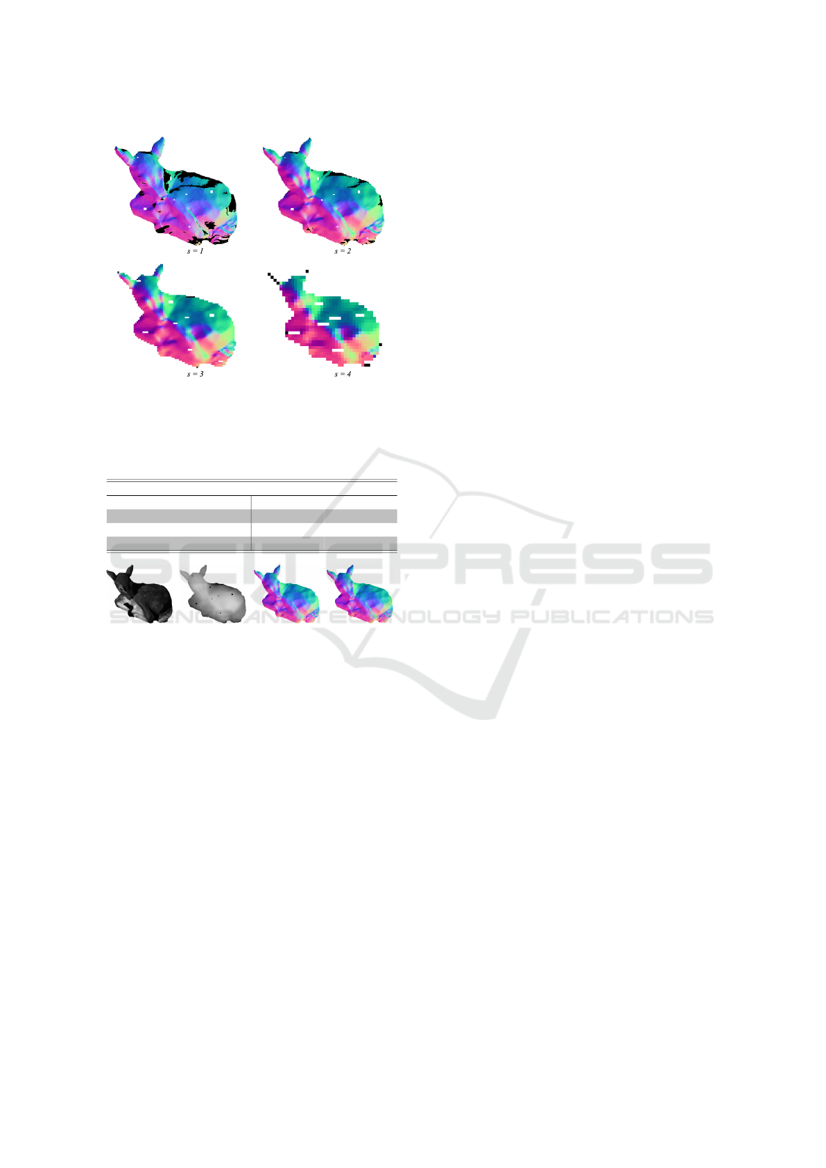
Figure 4: The estimated surface normal vectors for an in-

complete depth map. The white regions inside the object

demonstrate the areas where depth information is missing.

Table 1: Chosen neighbors according to the gradient direc-

tion. (𝑥, 𝑦) is the spatial location of a pixel of interest 𝑝

𝑖

Angles in degrees Neighbour locations

◦

, 45

◦

) [180

◦

, 225

◦

) (𝑥 − 1, 𝑦 + 1) (𝑥 + 1, 𝑦 − 1)

[45

◦

, 90

◦

) [225

◦

, 270

◦

) (𝑥 − 1, 𝑦) (𝑥 + 1, 𝑦)

[90

◦

, 135

◦

) [270

◦

, 315

◦

) (𝑥 − 1, 𝑦 − 1) (𝑥 + 1, 𝑦 + 1)

[135

◦

, 180

◦

) [315

◦

, 360

◦

] (𝑥, 𝑦 − 1) (𝑥, 𝑦 +1)

Figure 5: Estimation of normals from an easy case of in-

complete depth maps. (Left-to-right) Baseline shading, in-

complete depth map, ground truth, and estimated normals.

We extract the gradient directions from the shad-

ing element by using the gradient angle, to guide the

surface normal estimation procedure for incomplete

depth maps. In a 3 × 3 neighborhood, the two neigh-

bors in the same gradient direction are averaged to ﬁll

the missing surface normals (Table 1). In case only

one informative neighbor is present it is directly used

as the surface normal estimate. When no information

is present in both neighbors, estimation is performed

in other scales. Afterwards, the same procedure used

for complete depth maps is applied. Subsequently, a

small Gaussian smoothing operation with a standard

deviation of 0.8 is applied. An example of estimating

the normals from an incomplete depth map is given in

Fig.5.

It is also worth mentioning here that instead of us-

ing a gradient-guided approach, inpainting methods

could also be preferred. However, during our exper-

iments, we observed that such methods result in less

satisfying outcomes as presented in Appendix B.

3 EXPERIMENTS AND

DISCUSSION

We compared the performance of the proposed

method with the following geometry-based

algorithms; baseline, bicubic interpolation,

angle-weighted averaging (Klasing et al., 2009),

triangle-weighted averaging (Klasing et al., 2009),

SIRFS (Barron and Malik, 2014), and 3F2N (Fan

et al., 2021), which are brieﬂy explained in Sec. 1

(for details of the baseline, bicubic interpolation,

angle-weighted averaging, and triangle-weighted

averaging methods please refer to Appendix C). All

algorithms are used in their default settings without

any modiﬁcation or optimization. It is worth men-

tioning here that for the 3F2N method ﬁxed camera

parameters are used since the MIT-Berkeley Intrinsic

Images dataset does not provide camera speciﬁcs for

the scenes.

We carried out the statistical comparisons for com-

plete depth maps on the MIT-Berkeley Intrinsic Im-

ages dataset (Barron and Malik, 2014), while we per-

formed analyses for incomplete depth maps on the

augmented version of the MIT-Berkeley Intrinsic Im-

ages dataset. Furthermore, we provide visual compar-

isons on the New Tsukuba Dataset, since it does not

contain ground truth surface normals (Martull et al.,

2012). We conducted all the experiments by using an

Intel i7 CPU @2.7 GHz Quad-Core 16GB RAM ma-

chine.

In the remainder of this section, we brieﬂy explain

the datasets, evaluation metrics, and discuss the out-

comes.

3.1 Datasets

MIT-Berkeley Intrinsic Images Dataset. Surface

normal estimation is a widely studied research ﬁeld,

yet quantitatively evaluating the performance of the

algorithms is challenging, due to the lack of ground

truth information in most of the existing datasets (Ulu-

can et al., 2022a). In order to benchmark our ap-

proach statistically, we used the MIT-Berkeley Intrin-

sic Images dataset (Barron and Malik, 2014), which

is an extended version of the MIT Intrinsic Images

dataset (Grosse et al., 2009). The MIT-Berkeley In-

trinsic Images dataset contains 20 diﬀerent scenes,

which contain a single masked object. For each scene,

the depth map and ground truth surface normals are

provided, which makes the MIT-Berkeley Intrinsic

Images dataset suitable for our experiments (Fig. 6).

Augmented MIT-Berkeley Intrinsic Images

Dataset. In order to analyze the performance of

the proposed approach in the case of incomplete

IMPROVE 2023 - 3rd International Conference on Image Processing and Vision Engineering

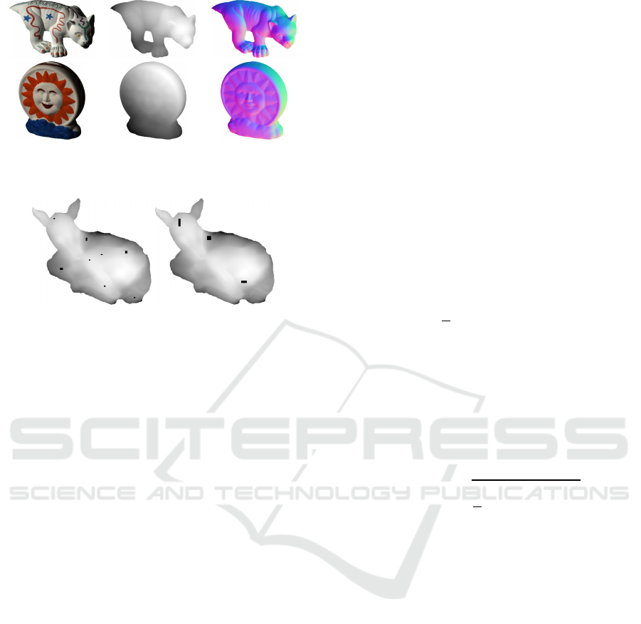
Figure 6: Examples from the MIT-Berkeley Intrinsic Im-

ages dataset. (Left-to-right) The scene, depth map, and the

surface normals.

Figure 7: The augmented version of the MIT-Berkeley In-

trinsic Images dataset with various diﬃculties. (Left-to-

right) Easy and hard cases.

depth maps, we modify the depth maps of the MIT-

Berkeley Intrinsic Images dataset by creating 2 sets,

namely, easy, and hard, where several areas of the

depth maps are randomly removed as shown in Fig. 7.

For the easy case, small-scale regions of the depth map

are removed, while for the hard case, large regions

containing up to 3000 pixels are deleted.

New Tsukuba Dataset. To present the perfor-

mance of our algorithm in scenes similar to the real

world, we also provide outcomes for scenes from the

New Tsukuba Dataset (Martull et al., 2012). This

dataset is rendered using various computer graphics

techniques and is composed of video sequences. The

dataset contains stereo pairs with ground truth depth

maps. Since ground truth surface normals are not

present in this dataset, we only provide visual com-

parisons. Furthermore, we are providing a video se-

quence, where we demonstrate our surface normal es-

timations for each frame of the New Tsukuba Dataset.

The video will be provided on the ﬁrst author’s web-

site upon publication.

3.2 Evaluation Metrics

Not only the datasets but also the evaluation metrics

have signiﬁcant importance in the ﬁeld of intrinsic im-

age decomposition (Barron and Malik, 2014). Since

the scores of all metrics may not coincide, many image

processing studies discuss that analyzing the perfor-

mance with multiple strategies is beneﬁcial (Fouhey

et al., 2013; Bonneel et al., 2017; Karakaya et al.,

2022; Garces et al., 2022). Thereupon, in order to

statistically evaluate the algorithms, we used two dif-

ferent metrics, namely, geodesic distance, and root

mean square error. We report the minimum, maxi-

mum, mean, median, best 25%, and worst 25% of the

errors.

The geodesic distance is the length of the shortest

path between the points on the surfaces along the man-

ifold. Since geodesic distance is responsive to slight

topology changes and noise, it is also independent of

the viewing angle of the observer (Pizer and Marron,

2017; Antensteiner et al., 2018). Thus, it is widely

used as a quality metric in many surface normal es-

timation studies. A lower geodesic distance between

the ground truth and the estimation means greater sim-

ilarity. The geodesic distance 𝐺𝐷𝐼𝑆 between the

ground truth 𝐧

𝑔𝑡

and the estimated surface normals

𝐧

𝑒𝑠𝑡

can be calculated as follows;

𝐺𝐷𝐼𝑆 =

𝑑



𝑖=1

𝑐𝑜𝑠

−1



𝐧

𝑔𝑡

𝑖

⋅ 𝐧

𝑒𝑠𝑡

𝑖





. (4)

Root mean square error is another commonly used

evaluation method in the ﬁeld of intrinsic image de-

composition (Fouhey et al., 2013). As in the geodesic

distance, a lower value of the root mean square error

indicates better results. The root mean square error

(𝑅𝑀𝑆𝐸) between the 𝐧

𝑔𝑡

and 𝐧

𝑒𝑠𝑡

can be computed

as follows;

𝑅𝑀𝑆𝐸 =







𝑑



𝑖=1



𝐧

𝑔𝑡

𝑖

− 𝐧

𝑒𝑠𝑡

𝑖



. (5)

3.3 Discussion

The statistical outcomes for the complete depth maps

are provided in Table 2. Our proposed algorithm out-

performs all the methods in each metric. The median

of both 𝐺𝐷𝐼𝑆 and 𝑅𝑀𝑆𝐸 are lower than their mean,

which indicates that our algorithm tends to produce re-

sults closer to the best outcomes rather than the worst

ones. We present the visual comparison on the MIT-

Berkeley Intrinsic Images dataset in Fig. 8. It can be

seen that the ﬁne details are preserved well even at the

edges.

While the performance gap between our method

and the existing averaging techniques may seem low

in terms of 𝐺𝐷𝐼𝑆, the advantage of our algorithm is

easily seen in Fig. 9, where complex scenes are used

instead of a single masked object. While the angle-

weighted averaging method cannot estimate surface

normals at ﬂat regions, our algorithm performs well

in such areas.

Multi-Scale Surface Normal Estimation from Depth Maps

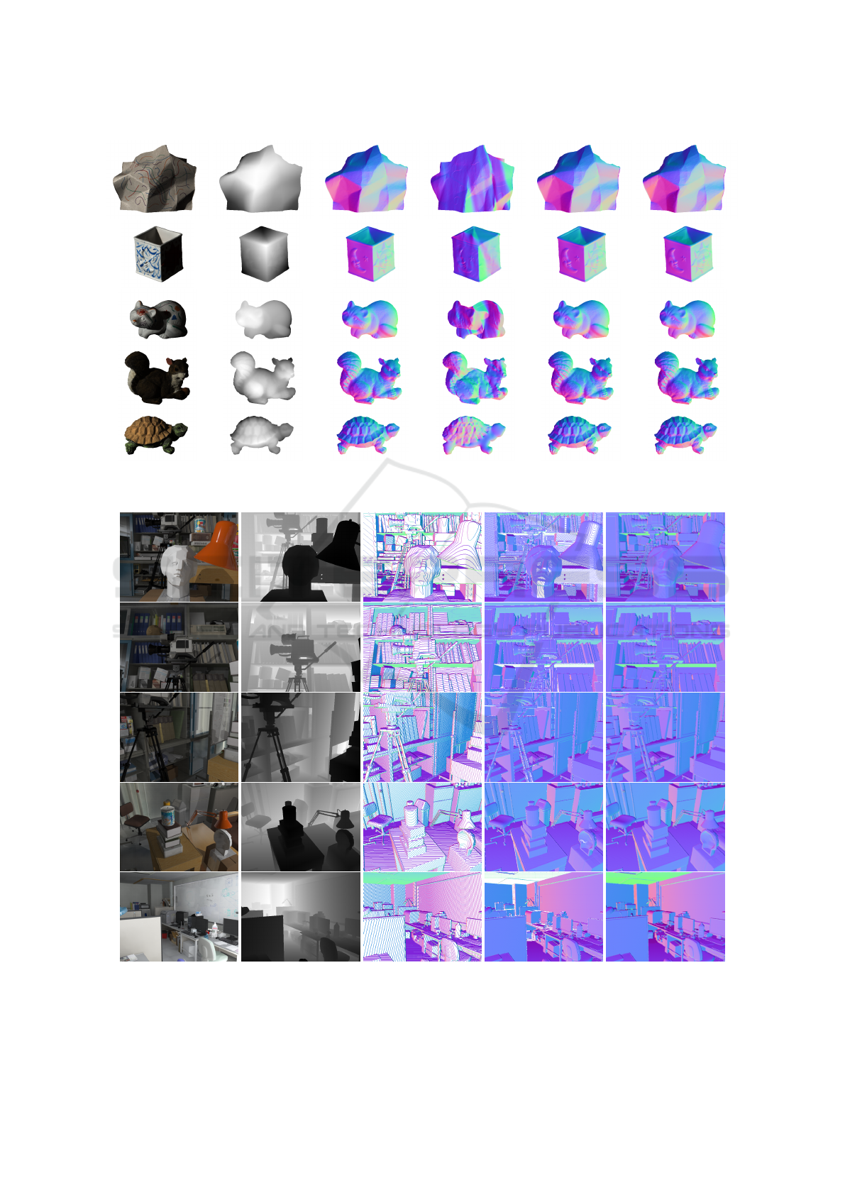
Figure 8: Visual comparison on the MIT-Berkeley Intrinsic Images dataset. (Left-to-right) The scene, depth map, ground

truth, and estimations of SIRFS, Area-Weighted, and proposed method.

Figure 9: Visual comparison on the New Tsukuba Dataset. (Left-to-right) The scene, depth map, and estimations of Angle-

Weighted, proposed without scale-space and proposed with scale-space. The white regions present the pixels, where surface

normals could not be computed. Note here that a diﬀerent threshold is used according to the range of this dataset.

IMPROVE 2023 - 3rd International Conference on Image Processing and Vision Engineering

Table 2: Statistical results on MIT-Berkeley Intrinsic Im-

ages dataset. Best scores are highlighted.

GDIS RMSE Run Time

Min. Mean Med. B.25% W.25% Max. Min. Mean Med. B.25% W.25% Max.

Baseline 0.996 0.999 0.999 0.998 1.000 1.000 0.783 0.968 0.953 0.854 1.094 1.270 0.059

Angle-Weighted 0.095 0.163 0.155 0.112 0.223 0.262 0.051 0.063 0.062 0.053 0.073 0 .083 3.942

Area-Weighted 0.095 0.163 0.155 0.111 0.223 0.262 0.046 0.056 0.055 0.048 0.066 0.073 3.813

Bicubic Interpolation 0.148 0.256 0.246 0.172 0.359 0.504 0.189 0.342 0.337 0.238 0.447 0.516 𝟎.𝟎𝟏𝟐

SIRFS 0.145 0.256 0.242 0.166 0.366 0.438 0.130 0.246 0.241 0.164 0.324 0.333 189.34

3F2N 0.218 0.379 0.377 0.271 0.494 0.563 0.400 0.490 0.500 0.414 0.572 0.626 0.040

Proposed without scale-space 0.096 0.163 0.155 0.112 0.223 0.263 0.046 0.056 0.055 0.048 0.066 0.073 0.762

Proposed with scale-space 𝟎.𝟎𝟗𝟏 𝟎.𝟏𝟔𝟎 𝟎.𝟏𝟓𝟑 𝟎.𝟏𝟎𝟖 𝟎.𝟐𝟐𝟎 𝟎.𝟐𝟓𝟗 𝟎.𝟎𝟑𝟕 𝟎.𝟎𝟒𝟗 𝟎.𝟎𝟒𝟖 𝟎.𝟎𝟑𝟗 𝟎.𝟎𝟔𝟏 𝟎.𝟎𝟔𝟒 1.422

Figure 10: Estimations from incomplete depth maps. (Left-

to-right) The depth map, ground truth surface normals, and

estimations of the proposed method.

We also compared our algorithm’s performance

without using the scale-space and directly applying

our computations in the ﬁnest scale. For this com-

parison, it is important to mention that even though

the statistical results especially in terms of 𝐺𝐷𝐼𝑆 do

not vary signiﬁcantly, the advantage of adopting scale-

space is clearly demonstrated in Fig. 9. When com-

plex scenes are of interest rather than a single masked

object, ﬂat regions cannot be ﬁlled and discontinuity at

edges is observed when surface normal computations

are not carried out in scale-space.

Furthermore, in Fig. 10 we provide visual out-

comes for the estimations obtained from incomplete

depth maps. Since the algorithms in Table 2 expect

complete depth maps as input it would not be fair

to investigate their performance on incomplete depth

maps, thus we only provide visual analysis for incom-

plete depth maps. Our approach is able to make accu-

rate estimations for both the easy and hard sets in the

dataset.

4 CONCLUSION

We present a simple yet eﬀective surface normal es-

timation strategy. Our method estimates surface nor-

mal vectors from both complete and incomplete depth

maps by taking advantage of scale-space. For com-

plete depth maps, while the initial estimations are car-

ried out in the ﬁnest scale of the pyramid, the regions

that cannot be estimated correctly in the ﬁrst scale are

ﬁlled from the coarser scales. For incomplete depth

maps, we follow the same procedure as in the com-

plete depth maps but with slight modiﬁcations. To ﬁll

missing regions in incomplete depth maps, we are tak-

ing advantage of the relationship between the surface

normals and the shading component of the scenes. We

compute the surface normals by guiding our algorithm

with the gradient directions obtained from the shad-

ing element. We benchmarked our method on the

well-known MIT-Berkeley Intrinsic Images dataset

and the New Tsukuba Dataset. Moreover, for incom-

plete depth maps, we modiﬁed the MIT-Berkeley In-

trinsic Images dataset. According to the experiments,

our approach can estimate surface normals eﬀectively

for both simple and complex scenes.

REFERENCES

Antensteiner, D., Štolc, S., and Pock, T. (2018). A re-

view of depth and normal fusion algorithms. Sensors,

18(2):431.

Awwad, T. M., Zhu, Q., Du, Z., and Zhang, Y. (2010). An

improved segmentation approach for planar surfaces

from unstructured 3d point clouds. Photogrammetric

Rec., 25:5–23.

Bansal, A., Russell, B., and Gupta, A. (2016). Marr re-

visited: 2D-3D alignment via surface normal predic-

tion. In Conf. Comput. Vision Pattern Recognit., pages

5965–5974, Las Vegas, NV, USA. IEEE.

Barron, J. T. and Malik, J. (2014). Shape, illumination, and

reﬂectance from shading. IEEE Trans. Pattern Anal.

Mach. Intell., 37(8):1670–1687.

Bonneel, N., Kovacs, B., Paris, S., and Bala, K. (2017).

Intrinsic decompositions for image editing. Comput.

Graph. Forum, 36:593–609.

Bornemann, F. and März, T. (2007). Fast image inpainting

based on coherence transport. J. Math. Imag. Vision,

28:259–278.

Cao, J., Chen, H., Zhang, J., Li, Y., Liu, X., and Zou, C.

(2018). Normal estimation via shifted neighborhood

for point cloud. J. Comput. Appl. Math., 329:57–67.

Criminisi, A., Pérez, P., and Toyama, K. (2004). Region

ﬁlling and object removal by exemplar-based image in-

painting. IEEE Trans. Image Process., 13:1200–1212.

Ebner, M. (2007). Color Constancy, 1st ed. Wiley Publish-

ing, ISBN: 0470058299.

Multi-Scale Surface Normal Estimation from Depth Maps

Ebner, M. and Hansen, J. (2013). Depth map color con-

stancy. Bio-Algorithms and Med-Systems, 9(4):167–

177.

Eigen, D. and Fergus, R. (2015). Predicting depth, surface

normals and semantic labels with a common multi-

scale convolutional architecture. In Int. Conf. Comput.

Vision, Santiago, Chile. IEEE.

Fan, R., Wang, H., Xue, B., Huang, H., Wang, Y., Liu, M.,

and Pitas, I. (2021). Three-ﬁlters-to-normal: An ac-

curate and ultrafast surface normal estimator. IEEE

Robot. Automat. Letters, 6(3):5405–5412.

Fouhey, D. F., Gupta, A., and Hebert, M. (2013). Data-

driven 3D primitives for single image understanding.

In Int. Conf. Comput. Vision, pages 3392–3399, Syd-

ney, NSW, Australia. IEEE.

Garces, E., Rodriguez-Pardo, C., Casas, D., and Lopez-

Moreno, J. (2022). A survey on intrinsic images: Delv-

ing deep into lambert and beyond. Int. J. Comput. Vi-

sion, 130:836–868.

Gouraud, H. (1971). Continuous shading of curved surfaces.

IEEE Trans. Computers, 100(6):623–629.

Grosse, R., Johnson, M. K., Adelson, E. H., and Free-

man, W. T. (2009). Ground truth dataset and base-

line evaluations for intrinsic image algorithms. In

Int. Conf. Comput. Vision, pages 2335–2342, Kyoto,

Japan. IEEE.

Harms, H., Beck, J., Ziegler, J., and Stiller, C. (2014). Ac-

curacy analysis of surface normal reconstruction in

stereo vision. In Intell. Vehicles Symp. Proc., pages

730–736, Dearborn, MI, USA. IEEE.

Hsu, H., Su, H.-T., Yeh, J.-F., Chung, C.-M., and Hsu, W. H.

(2022). SeqDNet: Improving missing value by se-

quential depth network. In Int. Conf. Image Process.,

pages 1826–1830, Bordeaux, France. IEEE.

Ioannou, Y., Taati, B., Harrap, R., and Greenspan, M.

(2012). Diﬀerence of normals as a multi-scale opera-

tor in unorganized point clouds. In Int. Conf. 3D Imag.

Model. Process. Visualization Transmiss., pages 501–

508, Zurich, Switzerland. IEEE.

Izadi, S., Kim, D., Hilliges, O., Molyneaux, D., Newcombe,

R., Kohli, P., Shotton, J., Hodges, S., Freeman, D.,

Davison, A., and Fitzgibbon, A. (2011). KinectFu-

sion: real-time 3D reconstruction and interaction us-

ing a moving depth camera. In Proc. Annu. ACM

Symp. User Interface Softw. Technol., pages 559–568,

Santa Barbara, CA, USA. ACM.

Jeon, J., Cho, S., Tong, X., and Lee, S. (2014). Intrinsic im-

age decomposition using structure-texture separation

and surface normals. In Eur. Conf. Comput. Vision,

pages 218–233, Zurich, Switzerland. Springer.

Karakaya, D., Ulucan, O., and Turkan, M. (2022). Image de-

clipping: Saturation correction in single images. Digit.

Signal Process., 127:103537.

Klasing, K., Althoﬀ, D., Wollherr, D., and Buss, M. (2009).

Comparison of surface normal estimation methods for

range sensing applications. In Int. Conf. Robot. Au-

tomat., pages 3206–3211, Kobe, Japan. IEEE.

Kwon, H., Tai, Y.-W., and Lin, S. (2015). Data-driven depth

map reﬁnement via multi-scale sparse representation.

In Conf. Comput. Vision Pattern Recognit., pages 159–

167, Boston, MA, USA. IEEE.

Li, B., Shen, C., Dai, Y., Van Den Hengel, A., and He, M.

(2015). Depth and surface normal estimation from

monocular images using regression on deep features

and hierarchical CRFs. In Conf. Comput. Vision Pat-

tern Recognit., pages 1119–1127, Boston, MA, USA.

IEEE.

Li, K., Zhao, M., Wu, H., Yan, D.-M., Shen, Z., Wang,

F.-Y., and Xiong, G. (2022). GraphFit: Learn-

ing multi-scale graph-convolutional representation for

point cloud normal estimation. In Eur. Conf. Comput.

Vision, pages 651–667, Tel Aviv, Israel. Springer.

Martull, S., Peris, M., and Fukui, K. (2012). Realistic cg

stereo image dataset with ground truth disparity maps.

In ICPR Workshop TrakMark2012, volume 111, pages

117–118.

Mitra, N. J. and Nguyen, A. (2003). Estimating surface nor-

mals in noisy point cloud data. In Proc. Annu. Symp.

Comput. Geometry, pages 322–328, San Diego, CA,

USA. ACM.

Pizer, S. M. and Marron, J. (2017). Object statistics on

curved manifolds. In Statistical Shape Deformation

Anal., pages 137–164. Elsevier.

Saracchini, R. F. V., Stolﬁ, J., Leitão, H. C. G., Atkinson,

G. A., and Smith, M. L. (2012). A robust multi-

scale integration method to obtain the depth from gra-

dient maps. Comput. Vision Image Understanding,

116(8):882–895.

Silberman, N., Hoiem, D., Kohli, P., and Fergus, R.

(2012). Indoor segmentation and support inference

from RGBD images. In Eur. Conf. Comput. Vision,

pages 746–760, Florence, Italy. Springer.

Ulucan, D., Ulucan, O., and Ebner, M. (2022a). IID-

NORD: A comprehensive intrinsic image decomposi-

tion dataset. In Int. Conf. Image Process., pages 2831–

2835, Bordeaux, France. IEEE.

Ulucan, O., Ulucan, D., and Ebner, M. (2022b). BIO-CC:

Biologically inspired color constancy. In BMVC, Lon-

don, UK. BMVA Press.

Ulucan, O., Ulucan, D., and Ebner, M. (2022c). Color

constancy beyond standard illuminants. In Int. Conf.

Image Process., pages 2826–2830, Bordeaux, France.

IEEE.

Zeng, J., Tong, Y., Huang, Y., Yan, Q., Sun, W., Chen, J.,

and Wang, Y. (2019). Deep surface normal estima-

tion with hierarchical RGB-D fusion. In Conf. Com-

put. Vision Pattern Recognit., Long Beach, CA, USA.

IEEE/CVF.

Zhang, Y. and Funkhouser, T. (2018). Deep depth comple-

tion of a single rgb-d image. In Conf. Comput. Vision

Pattern Recognit., pages 175–185, Salt Lake City, UT,

USA. IEEE/CVF.

Zhou, J., Huang, H., Liu, B., and Liu, X. (2020). Nor-

mal estimation for 3d point clouds via local plane con-

straint and multi-scale selection. Comput. Aided Des.,

129:102916.

IMPROVE 2023 - 3rd International Conference on Image Processing and Vision Engineering

APPENDIX A

Determination of the Threshold. As mentioned in

Sec. 2, the surface normal vectors are computed only

at pixels, where there is a small change in depth. In

other words, to compute the surface normals without

missing the ﬁne details in the depth maps, a thresh-

old value that respects the slight distances between the

neighbouring pixels should be considered. Hence, we

minutely investigate diﬀerent threshold values with re-

spect to their RMSE, and GDIS scores over the en-

tire MIT-Berkeley Intrinsic Images dataset. When we

analyze the errors with respect to the threshold val-

ues (Fig. 11), it is observable that the diﬀerence be-

tween the errors does not signiﬁcantly vary. We see

from Fig. 11 that the best-performing threshold is be-

tween 0.5 and 1.3. When we analyze the estimated

surface normals by considering each threshold, for

each given scene, we observed that the best outcomes

are obtained at the value of 0.9, while using a thresh-

old of 0.5 and 1.0 results in estimations with signiﬁ-

cant errors in some of the scenes. Hence for the ﬁnest

scale, the threshold value is determined as 0.9. For the

coarser scales, since the image is down-sampled with

a ratio of 1∕4, we increase the threshold value 4 times

with respect to the threshold of the previous scale.

APPENDIX B

Analysis of Filling Missing Pixels in Depth Maps

before Estimating Surface Normals. We observed

during our experiments that in case the missing pixels

in the depth map are ﬁlled and the surface normals

are estimated from this data the outcomes have lower

accuracy than using our proposed algorithm for

incomplete depth maps. In Fig. 12 we present the

outcomes of our observation.

Comparison of Inpainting Methods and Gradient-

Guided Filling. For the incomplete depth maps, we

compare our method with its variations, where we

used inpainting methods instead of gradient-guided

ﬁlling. One of the methods we tested is the exemplar-

based inpainting method, which segments the image

into target and source regions, where the target

includes the pixels that need to be ﬁlled (Criminisi

et al., 2004). For a patch from the target region, the

most similar patch in the source area is found and

copied to the target patch. Another method we used

is the coherency-based inpainting approach, which

takes advantage of the coherent neighboring pixels,

whose values are known (Bornemann and März,

2007). The last method we compare our gradient-

Figure 11: Analysis on the determination of the threshold.

Figure 12: Analysis of ﬁlling missing pixels in depth maps.

(Top-to-bottom) Incomplete depth map, ﬁlled depth map,

ground truth normals, normals estimated from the ﬁlled

depth map, and estimation of the proposed method.

guided ﬁlling procedure to is the interpolation-based

approach, which performs interpolation by starting at

the boundary of a missing area (MATLAB regionﬁll).

In Fig. 13, we show examples from the easy and

hard sets. Our gradient-guided ﬁlling approach results

in more accurate outcomes than the other methods.

Multi-Scale Surface Normal Estimation from Depth Maps

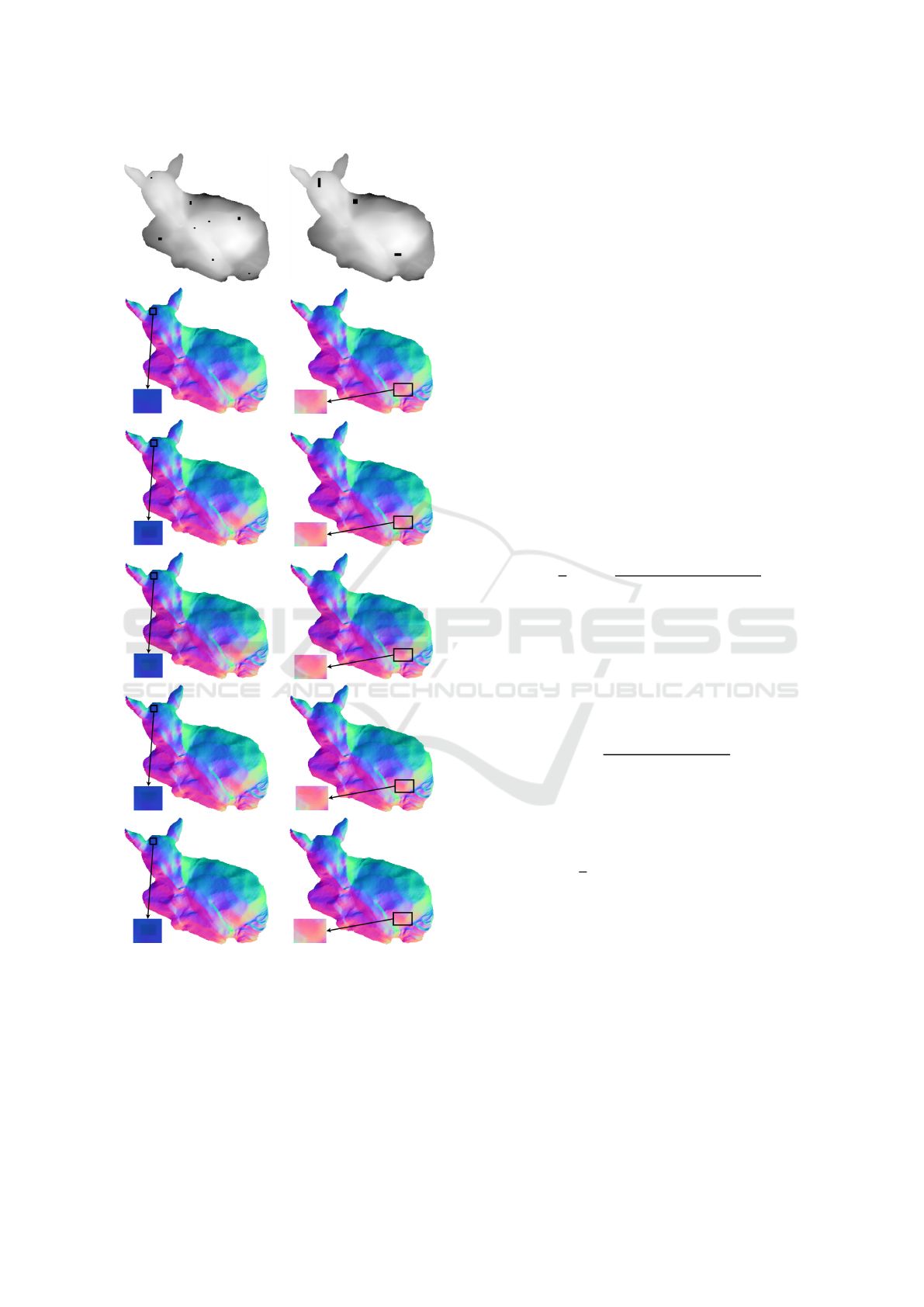
Figure 13: Comparison of inpainting methods. (Left-to-

right) Examples from the easy and hard set. (Top-to-bottom)

The depth map with missing pixels, ground truth surface

normal vectors, outcomes of the exemplar-based inpaint-

ing method (Criminisi et al., 2004), coherency-based in-

painting method (Bornemann and März, 2007), bicubic in-

terpolation, and proposed gradient-guided ﬁlling approach.

The missing regions are more accurately estimated with the

gradient-guided ﬁlling method.

APPENDIX C

Baseline Approach. The baseline approach computes

the surface normal vector for a pixel 𝑝

𝑖

from its con-

secutive neighbours in the horizontal and vertical di-

rections as follows;

𝐧

𝑖

𝑥

= 𝑝

(𝑖+1)

𝑥

− 𝑝

𝑖

𝑥

(6)

𝐧

𝑖

𝑦

= 𝑝

(𝑖+1)

𝑦

− 𝑝

𝑖

𝑦

(7)

𝐧

𝑖

𝑧

= −1. (8)

Bicubic Interpolation. The surface normals are

computed by applying bicubic interpolation on the

depth map, and using quadratic extrapolation on

the boundaries. After bicubic ﬁt is carried out, the

diagonal vectors are obtained and crossed to estimate

surface normals (MATLAB surfnorm).

Averaging Methods. There are several varia-

tions of the averaging method. The general equation

for averaging can be represented as follows;

𝐧

𝑖

𝑘



𝑗=1

𝑤

𝑖

𝑗

[ℎ

𝑖

𝑗

− 𝑝

𝑖

] × [ℎ

𝑖

𝑗+1

− 𝑝

𝑖

]

[ℎ

𝑖

𝑗

− 𝑝

𝑖

] × [ℎ

𝑖

𝑗+1

− 𝑝

𝑖

]

(9)

where, ℎ

𝑖

𝑗

and ℎ

𝑖

𝑗+1

are neighbours of 𝑝

𝑖

, 𝑤

𝑖

𝑗

is the

weight, which is 1 in the classical method.

For the angle-weighted averaging method 𝑤

𝑖

𝑗

the angle between the crossed vectors and can be com-

puted as follows;

𝑤

𝑖

𝑗

= 𝑐𝑜𝑠

−1



ℎ

𝑖

𝑗

− 𝑝

𝑖

, ℎ

𝑖

𝑗+1

− 𝑝

𝑖



ℎ

𝑖

𝑗

− 𝑝

𝑖

ℎ

𝑖

𝑗+1

− 𝑝

𝑖





. (10)

For the triangle-weighted averaging method, the

surface normal of each triangle is weighted according

to its area’s magnitude as follows;

𝑤

𝑖

𝑗



[ℎ

𝑖

𝑗

− 𝑝

𝑖

] × [ℎ

𝑖

𝑗+1

− 𝑝

𝑖

]



. (11)

IMPROVE 2023 - 3rd International Conference on Image Processing and Vision Engineering