An Automatic Ant Counting and Distribution Estimation System Using

Convolutional Neural Networks

Mateus Coelho Silva

1 a

, Breno Henrique Felisberto

2 b

, Mateus Caldeira Batista

3 c

Andrea Gomes Campos Bianchi

1 d

, Servio Pontes Ribeiro

3 e

and Ricardo Augusto Rabelo Oliveira

1 f

Computing Department, Universidade Federal de Ouro Preto, Ouro Preto, Brazil

General Biology Department, Universidade Federal de Vic¸osa, Vic¸osa, Brazil

Biology Department, Universidade Federal de Ouro Preto, Ouro Preto, Brazil

Keywords:

Convolutional Neural Networks, Ant Ecology, Population Distribution.

Abstract:

A relevant challenge to be tackled in ecology is comprehending collective insect behaviors. This understanding

signiﬁcantly impacts the understanding of nature, as some of these ﬂocks are the most extensive cooperative

units in nature. A part of the difﬁculty in tackling this challenge comes from reliable data sampling. This work

presents a novel method to understand the quantities and distribution of ants in colonies based on convolutional

neural networks. As this tool is unique, we created an application to create the marked dataset, created the ﬁrst

version of the dataset, and tested the solution with different backbones. Our results suggest that the proposed

approach is feasible to solve the proposed issue. The average coefﬁcient of determination R

with the ground

truth counting was 0.9783 using the MobileNet as the backbone and 0.9792 using the EfﬁcientNet V2B0 as

the backbone. The global average for the semi-quantitive classiﬁcation of each image region was 86% for the

MobileNet and 88% for the EfﬁcientNet V2-B0. There was no statistically signiﬁcant difference between both

cases’ average and median errors. The coefﬁcient of determination was close to the statistical signiﬁcance

threshold (p = 0.065). The application using the MobileNet as its backbone performed the task faster than the

version using the EfﬁcientNet V2-B0, with statistical signiﬁcance (p < 0.05).

1 INTRODUCTION

Understanding collective ant behaviors is a critical

challenge in ecology. Helanter

a et al. (Helanter

et al., 2009) assert that unicolonial ant populations are

the largest cooperative units in nature. They state that

these species can construct interconnected nests with

hundreds of kilometers. The authors also state that

understanding the dynamics of such colonies allows

the generation of valuable information for researchers

in this ﬁeld.

McGlynn (McGlynn, 2012) states that insect

colonies are mobile entities, moving nests through

their lifetime. The authors state that understand-

https://orcid.org/0000-0003-3717-1906

https://orcid.org/0000-0002-9799-1941

https://orcid.org/0000-0002-2591-8315

https://orcid.org/0000-0001-7949-1188

https://orcid.org/0000-0002-0191-8759

https://orcid.org/0000-0001-5167-1523

ing the aspects that drive this mobility enforces the

knowledge of several aspects of the studied species,

such as the understanding of its genetics, life-history

evolution, and the role of competition. More specif-

ically, the authors afﬁrm that the migration patterns

are often unclear in the case of ants.

Regarding the methods of understanding the mi-

gration patterns of ant colonies, Hakkala et al.

(Hakala et al., 2019) state that reliable data capture

of the colony motion is needed. They also state that

this data can be combined with environmental data to

understand the role of the context in their migration.

For this matter, technological solutions are a way to

improve data gathering and develop novel solutions

towards this goal.

The topic of planning experiments towards this

goal is also assessed by Majer and Heterick (Majer

and Heterick, 2018). The authors state that long-

term monitoring is essential for invertebrate studies.

This aspect also enforces that developing novel tech-

Silva, M., Felisberto, B., Batista, M., Bianchi, A., Ribeiro, S. and Oliveira, R.

An Automatic Ant Counting and Distribution Estimation System Using Convolutional Neural Networks.

DOI: 10.5220/0011968900003467

In Proceedings of the 25th International Conference on Enterprise Information Systems (ICEIS 2023) - Volume 1, pages 547-554

ISBN: 978-989-758-648-4; ISSN: 2184-4992

 2023 by SCITEPRESS – Science and Technology Publications, Lda. Under CC license (CC BY-NC-ND 4.0)

547

Figure 1: Designed solution.

nological tools toward this goal positively impacts re-

searchers in this area.

Thus, this work explores how to create a novel tool

that allows researchers to evaluate the dynamics in

ant colonies. We expect to extract information about

quantities and distribution using the created technol-

ogy. Figure 1 summarizes the proposed solution. We

aimed to create a system that automatically counts

ants present in the solution. The solution also allows

an understanding of how the ants are approximately

distributed in the scene.

The main contribution of this work is:

• A method to estimate the counting and distribu-

tion of ants in a dense scene.

Additional contributions from this text are:

• A tool to generate a dot map-based structured

dataset for sparse and dense scenes;

• An evaluation of different convolutional neural

network backbones to perform the proposed task;

The remainder of this text is organized as follows:

In Section 2, we studied the theoretical references

around the counting on dense and sparse scenes. Sec-

tion 3 discusses some related works found in the lit-

erature and how they differ and relate to our proposal.

We present the materials and methods used to create

the solution in Section 4 and discuss the results in

Section 5. Finally, we display our conclusions, dis-

cussions, and future works in Section 6.

2 THEORETICAL REFERENCES

In this context, we want to determine both the number

of individuals and their geometric location. In some

cases, the counting is sparse, while often, the process

is determining the counting in a dense scene. Thus,

we require an understanding of counting processes in

sparse and dense scenes.

According to Kahn et al. (Khan and Basalamah,

2021), the methods to perform this task is divided

into detection-based methods and regression-based

methods. On the one hand, regression-based meth-

ods extract features from the images and try to per-

form a regression using this data. On the other hand,

detection-based methods try to identify each individ-

ual instance.

Sindagi and Patel (Sindagi and Patel, 2018) as-

sess that counting crowds using these methods has

several applications, such as behavior analysis, con-

gestion analysis, anomaly detection, and event de-

tection. These high-level tasks are helpful in hu-

man beings’ context but can also transport to under-

standing ecological behaviors, as presented in the pre-

vious section. These authors classify the methods

among detection-based, regression-based, and den-

sity estimation-based. The latter category comes from

the understanding that spatial information might be as

important as counting the number of individuals.

A way of generating data for these applications is

through dot annotation maps. For instance, Wan et

al. (Wan et al., 2020) employ this technique for dense

crowd counting. In their case, they transform this map

into a density map, which works as a baseline for

density estimation. They employ a two-dimensional

gaussian kernel function to generate densities from

these dot annotation maps.

In this work, we also employ a ﬁrst stage based

on a dot annotation map to generate the dense-object

counting dataset for ants counting. Then, we employ

a semi-quantitative method to estimate the density of

ants in each region of the image. Finally, we use this

local estimation to estimate the total number of indi-

vidual ants per image.

3 RELATED WORKS

Some authors employed artiﬁcial intelligence meth-

ods for counting arthropods. Schneider et al. (Schnei-

der et al., 2022) used computer vision and machine

learning to count and classify arthropods. They rely

on clean Petri dish images with arthropods, using

computer vision to segment and count the number of

individuals. Then, they employ convolutional neural

networks to classify each individual. Although the

authors obtained a good result, this method does not

apply to dense scenes due to overlap.

Tresson et al. (Tresson et al., 2021) proposed em-

ploying a combination of SSD and Faster RCNN to

ICEIS 2023 - 25th International Conference on Enterprise Information Systems

548

identify and classify small arthropods in an image.

They employ a hierarchical classiﬁer for the classi-

ﬁcation stage, using a step in which the objects are

classiﬁed among a superclass, then into subclasses.

This method is a different approach than the one em-

ployed in this work, as it displays a detection-based

method. Also, there is no discussion of whether the

proposed method works in dense scenes.

Bjerge et al. (Bjerge et al., 2022) developed a

real-time system to track insects. These authors em-

ploy the YOLOv3 algorithm to track and identify

sparse insects in an image in real time. Although

the authors want to study dynamics, this application

differs from the one presented in this work as it is

a detection-based method in a sparse scene. Our

objective approaches more regression- and density-

estimation-based techniques.

Eliopoulos et al. (Eliopoulos et al., 2018) devel-

oped a trap to count and identify crawling insects and

arthropods in urban environments. They created this

trap which captures the insects and arthropods, gener-

ating sparse images containing some individuals. Al-

though these authors also obtained good results from

their experiment, the exact nature of their work differs

from what is presented in this text.

Our research found no authors who employed

regression- and density-estimation-based techniques

in this context. Also, we did not observe researchers

proposing technological solutions aiming at the dis-

tribution and counting in ant or other arthropod

colonies. Another indicator for this case is the lack

of published datasets to perform this task. Therefore,

we understand that there is a notable degree of inno-

vation in the produced solution.

4 METHODOLOGY

In the previous sections, we assessed the importance

and novelty of the proposed solution. As demon-

strated, there is no precedent in producing a simi-

lar solution in the literature. In this section, we ex-

plore the details of the proposed solution. We initially

overview the proposed solution in detail. Then, we

will explore the dataset creation tool. We also assess

the backbone training process, presenting some de-

tails of the training algorithm. Finally, we display the

evaluation metrics for each stage.

4.1 Solution Overview

The proposed solution tries to estimate the number

of ants present in each area of the image. For this

matter, the employed algorithm has four main steps

to estimate the number of ants from a picture. The

steps involved in this algorithm are:

1. Transform the image size to 1024x1024;

2. Divide the image into a grid of squares of size

128x128;

3. Evaluate semi-quantitatively how many ants are

present in each square;

4. Submit the results to an approximation formula

for estimation;

The ﬁrst step is converting the image size to

1024x1024 pixels. This step helps evaluate hetero-

geneous images, as our created dataset has images

of various resolutions. With this step, we homoge-

nize the number of evaluated regions for each image,

leading to the second step. In this step, we divide

the image into regions of 128x128 pixels. This ini-

tial processing helps to create 64 regions of evalu-

ation on each image. Each region is independently

evaluated by the deep learning model and is classiﬁed

among ten classes representing quantity bands from 0

to 45 ants per region. After this evaluation, we use

the model output for each chunk to reconstruct the

image considering the density of each region and per-

form the counting. Figure 2 represents the complete

overview of the proposed solution.

Figure 2: Proposed system overview.

As previously discussed, this work is an inno-

vative approach to this task. Thus, some steps are

required to complete this task. We initially need

a dataset produced by researchers in ecology. This

dataset requires a computational tool to organize and

structure the data. Then, some steps are required to

train the AI, including choosing a backbone model

An Automatic Ant Counting and Distribution Estimation System Using Convolutional Neural Networks

549

for the CNN. Finally, we need to establish metrics to

evaluate the proposed work.

4.2 Dot Map Generation

As stated before, this is an unsolved problem with no

open dataset. Thus, we created a tool to generate a

structured dataset. Similarly to the dataset used by

Wan et al. (Wan et al., 2020), we chose to create a dot

map representing the presence of individual ants on

each part of the image. We produced a Guided User

Interface (GUI) to perform the task. Figure 3 displays

a software workﬂow diagram.

Figure 3: Dataset generation software diagram.

There are three main screens in the program. The

ﬁrst one is the initial screen, in which the user con-

ﬁgures the input and output folders. In this screen,

there are two path selection inputs. The ﬁrst one re-

ceives the path for the folder containing the images

the user wants to count. The second one receives the

path where the user wants the structured CSV ﬁle con-

taining the markings’ information output. The dataset

is recorded in a ﬁle named “result.csv” on the output

path.

The second one is the counting screen, where the

users mark a dot on each unit they want to mark.

This screen has several commands. The users must

click on the screen where they want their dot to be.

The software will store the coordinates and paint a

red dot on each marking. If users want to erase the

latest marking, they should click the ”Undo” button.

When they are done with the markings on the image,

they can click ”Next,” causing the program to store

the markings on disk and load the following image.

The end screen, in which the program warns the

user they have marked all images and ﬁnishes the ex-

ecution. It only gives the option to end the execution.

The laboratory members annotated 134 images us-

ing this program, producing the dot maps for sparse

and dense scenes of ant colonies. The image with the

least number of ants has one, while the image with the

most has 460 ants. Figure 4 displays a boxplot of the

number of ants per image, demonstrating that several

images are distributed from sparse to dense scenes.

Figure 4: Number of Ants per Image Distribution.

With these structured annotations, we reshaped

each image into the 1024x1024 format, translating

the markings into the correct coordinates. This step

allowed each image to generate 64 regions containing

various numbers of ants. To create a semi-quantitative

representation that suits the task, we divided them into

ten classes. The ﬁrst class is for regions with no ants.

Then, each class represents a band of up to ﬁve ad-

ditional ants (1-5, 6-10, 11-15, etc.). The ﬁnal class

represents the most ants per region, which is 45. Any

region with more than 45 ants would be reduced to

this maximum. The 134 annotated images produced

8576 frames for training the semi-quantitative classi-

ﬁcation convolutional neural network.

4.3 AI Model Training and Counting

System

As stated before, we started this stage with 8576 im-

ages of regions to be classiﬁed into ten classes. We

used a convolutional neural network (CNN) as the

engine to perform this task. We explored two high-

performance CNNs as backbones to this method for

testing purposes. The ﬁrst is the MobileNet (Howard

et al., 2017), and the second is the EfﬁcientNet V2-

ICEIS 2023 - 25th International Conference on Enterprise Information Systems

550

B0 (Tan and Le, 2021). Both models are lightweight

CNNs, ideal for performing high-demanding tasks

and later aiming at embedded solutions. The training

hardware has an i5-9600K CPU and 32 GB of RAM.

It also has an NVidia GeForce RTX 2060 Super video

card, supporting GPU acceleration for machine learn-

ing.

The created model has an input layer, the back-

bone without the ﬁnal classiﬁcation layer, a dense

layer with 32 neurons and linear activation function,

and a ﬁnal dense classiﬁcation layer with ten neurons

and “softmax” activation function. Both dense layers

use L1 kernel regularization with 0.01 as λ factor.

From the initial 8576 images, we separated 80%

for training, 10% for validation, and 10% for test-

ing. As the dataset is not balanced, we used the class

weights as a tool to enhance the classiﬁcation in the

least-represented classes. We used the square root of

the initial balanced class weights to keep the weights

apart from exceedingly high or low values. We em-

ployed the Adam loss function for this training.

We began the training with a learning rate of 1 ×

−4

, which was reduced to 10% of each value when

ﬁnding plateaus of 5 epochs. Finally, the algorithm

will stop early when ﬁnding a plateau of 15 epochs in

the validation loss.

After training the CNNs, the counting system con-

siders the output of these networks for each region

on the image to perform the counting. The output

of the classiﬁcation model is an integer from 0 to 9,

obtained from the argmax function, which evaluates

which class had the highest classiﬁcation probability.

Letting C

be the classiﬁcation integer obtained from

the i-th region from an image on the dataset, the num-

ber of ants N

on that region is:

• N

= 0, if C

= 0;

• N

= 1, if C

= 1;

• N

= 4 ×C

, if 2 ≤ C

≤ 6;

• N

= 5 ×C

, if C

> 6.

The number of ants per image A, considering each

i region on the image, is given by the equation:

A =

∑

(1)

4.4 Evaluation Metrics

After settling the methods for predicting the number

of ants on each part of the dataset, we need to estab-

lish evaluation metrics for each stage of the method.

Mainly, we focus on the two critical parts of the algo-

rithm: the region classiﬁcation and the counting. The

region classiﬁcation, as the name suggests, is a clas-

siﬁcation problem. The counting characterizes as a

regression problem.

As stated, the ﬁrst stage is a classiﬁcation prob-

lem. For this matter, we used the traditional machine-

learning metrics towards classiﬁcation: Precision, Re-

call, and F1-Score. They are deﬁned by the True Pos-

itive (T P), False Positive (FP), and False Negative

(FN) samples from each class. The equations which

deﬁne each metric are:

Precision =

T P

T P + FP

(2)

Recall =

T P

T P + FN

(3)

F1-Score = 2 ×

Precision × Recall

Precision + Recall

(4)

Besides these metrics, we also evaluated the

global average and the confusion matrix as quantita-

tive and qualitative indicators of the model function-

ing.

With the metrics deﬁned for the classiﬁcation

problem, we also need to establish the metrics for the

regression. Typically, we use the coefﬁcient of de-

termination R

as an indicator for the quality of re-

gressions. This coefﬁcient is deﬁned from the resid-

ual sum of squares SS

and the total sum of squares

. Ideally, the count would approach the function

f (x) = x, where f (x) is the number of ants counted

by the AI, and x is the ground-truth value.

The residual sum of squares can be deﬁned using

as the ground truth for the n-th image and

) as

the model output. The equation which represents the

is:

∑

(

) − x

) (5)

Similarly, the total sum of squares can be calcu-

lated from the mean output value

f and all

)

values obtained as the model outputs. The equation

which represents the SS

is:

∑

(

) −

f ) (6)

The equation gives the coefﬁcient of determina-

tion R

= 1 −

(7)

We evaluated the coefﬁcient of determination in

10 executions for each backbone to determine if there

An Automatic Ant Counting and Distribution Estimation System Using Convolutional Neural Networks

551

is any statistically signiﬁcant difference between the

models. We also compared the average error, the stan-

dard deviation of the error, and the median of the error

for both backbones. Finally, we compared the time

taken for each prediction on the complete dataset us-

ing both CNNs. We evaluated the statistical differ-

ences using the paired t-Test.

5 EXPERIMENTAL RESULTS

After deﬁning the metrics to evaluate the system, we

performed the training and testing with the proposed

algorithm. The initial evaluation comes from the

backbone CNNs. Our initial approach is quantitative.

Table 1 compresses the classiﬁcation metrics for the

tests evaluating the MobileNet as the backbone. The

global accuracy was circa 86%. The metrics display

a reduction in the quality of the model when predict-

ing the higher-density classes. These results are due

to the lower presence of samples of this size.

As the problem comes from a semi-quantitative

approach, it is also necessary to evaluate how the

misses can affect the result using a more qualitative

approach. For this matter, we evaluate the confusion

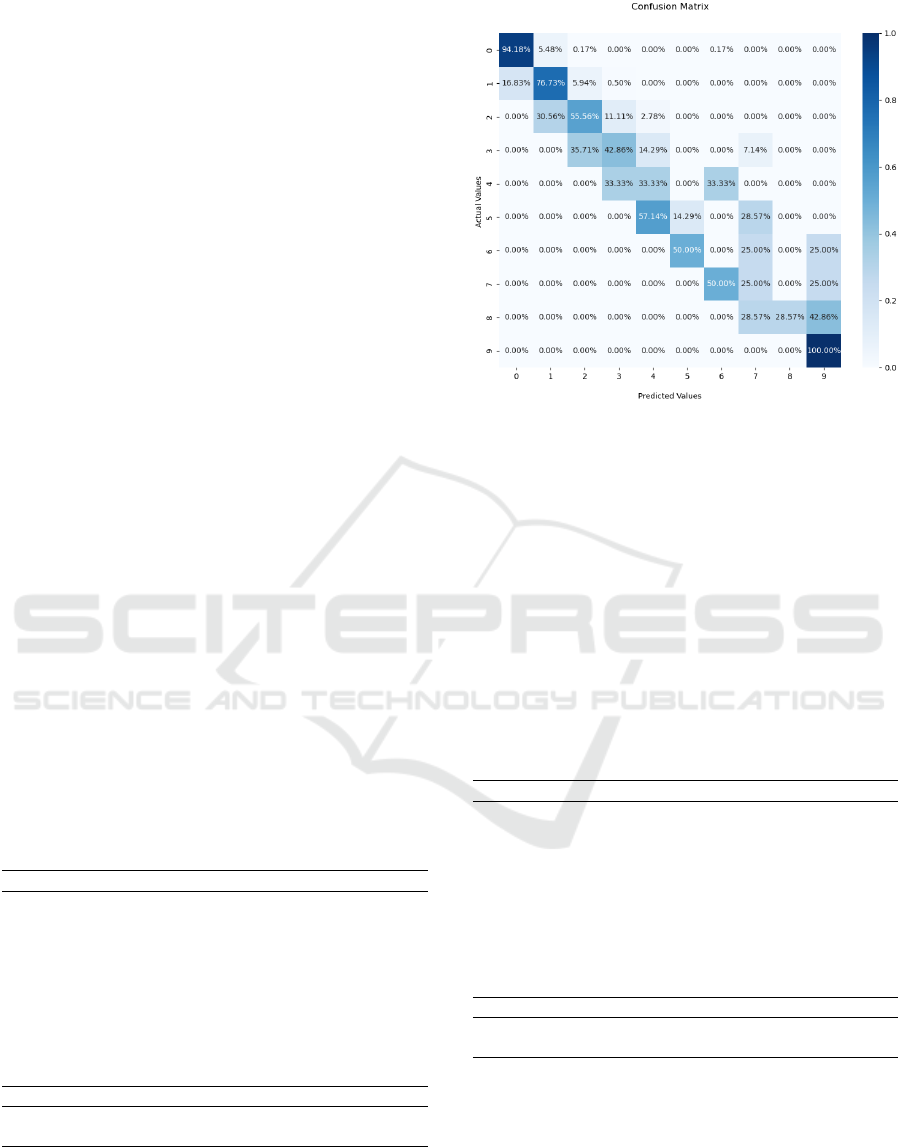
matrix as a source of information. Figure 5 displays

the confusion matrix obtained using the MobileNet as

the backbone. As the image suggests, most errors are

above or below one class, resulting in errors contained

within ﬁve ants.

These initial results suggested that the proposed

method can reach an acceptable estimation to com-

plete the main counting tasks. Additionally, it sug-

gests the capability of recognizing the density of ants

in each area with enough quality.

Table 1: MobileNet classiﬁcation metrics.

Precision Recall F1-score Support

0 0.92 0.96 0.94 584

1 0.81 0.70 0.75 202

2 0.56 0.67 0.61 36

3 0.58 0.50 0.54 14

4 0.40 0.67 0.50 3

5 0.50 0.29 0.36 7

6 0.17 0.25 0.20 4

7 0.25 0.25 0.25 4

8 0.60 0.43 0.50 7

9 0.50 0.67 0.57 3

Accuracy 86%

Macro avg. 0.53 0.54 0.52 864

Weighted avg. 0.86 0.86 0.86 864

The next step is evaluating the EfﬁcientNet V2-B0

using the same metrics. In this case, the global accu-

racy was 88%. Table 2 displays the obtained results

from training this network. Although it has a higher

Figure 5: Confusion Matrix for the MobileNet.

global average, it initially displays some issues with

some classes. As in the previous case, most issues are

related to the least represented classes.

The similarities and differences also display the

need for another qualitative evaluation using the con-

fusion matrix. Figure 6 displays the confusion matrix

evaluating the test set. Again, in this case, most er-

rors happen in classes close to the correct classiﬁca-

tion, indicating the feasibility of using this tool in the

counting algorithm. The following steps are to eval-

uate the behavior of these methods within the context

of the counting application.

Table 2: EfﬁcientNet V2-B0 classiﬁcation metrics.

Precision Recall F1-score support

0 0.94 0.96 0.95 584

1 0.84 0.78 0.81 202

2 0.72 0.72 0.72 36

3 0.64 0.50 0.56 14

4 0.14 0.33 0.20 3

5 0.12 0.14 0.13 7

6 0.12 0.25 0.17 4

7 0.00 0.00 0.00 4

8 0.50 0.43 0.46 7

9 0.50 0.33 0.40 3

Accuracy 88%

Macro avg. 0.45 0.45 0.44 864

Weighted avg. 0.88 0.88 0.88 864

As the former section suggests, the counting task

is similar to a regression problem. Nonetheless, we

know the ideal function we wanted the data to ﬁt.

Therefore, we developed our metrics demonstrated in

the former section considering the coefﬁcient of de-

termination to this ideal ﬁt function.

We executed ten stages of training and testing us-

ing the same dataset and separation using each back-

ICEIS 2023 - 25th International Conference on Enterprise Information Systems

552

Figure 6: Confusion Matrix for the EfﬁcientNet V2-B0.

bone. Our approach in this experiment is to demon-

strate if both systems work in an actual counting stage

and if there is any statistically signiﬁcant difference

from using each backbone model.

Initially, we evaluated the metrics using the Mo-

bileNet as the backbone. Table 3 displays the results

obtained from these tests. We can see that the results

are consistent, with an average error of circa ten ants.

The median error is circa eight ants. The average co-

efﬁcient of determination was 0.9783, consistent in

the ten runs, with a standard deviation of approxi-

mately 10

−3

. This result indicates the feasibility of

the tool in counting from sparse to dense scenes.

Table 3: Counting metrics for the MobileNet.

Median error Mean error SD error R

8 10.34 10.36 0.9774

8 10.61 10.61 0.9773

7.5 9.91 9.91 0.9797

7.5 10.61 10.69 0.9777

7.5 10.56 10.72 0.9766

7.5 10.17 10.23 0.9778

7 9.86 9.83 0.9799

7.5 10.00 10.22 0.9785

7 9.94 10.23 0.9787

7.5 10.17 10.43 0.9792

Average 7.5 10.22 10.32 0.9783

We also studied the metrics obtained using the Ef-

ﬁcientNet V2-B0 as the backbone. Table 4 displays

the results from the second set of tests. The results

also display consistent behavior, indicating that re-

placing the backbone also produced a feasible solu-

tion. The average coefﬁcient of determination was

0.9792 and consistent in the ten runs, with a standard

deviation of approximately 10

−3

. The average error

was circa ten ants, and the median error was circa

seven ants.

At ﬁrst, the results seem similar to the previous

tests, with some of them indicating a minor improve-

ment in the second set. When analyzing the data, it

did not support that this improvement was statistically

signiﬁcant. The only result which approached statis-

tically signiﬁcant improvement was the coefﬁcient of

determination R

, with the p-value of 0.065 using a

paired t-Test as the baseline.

Table 4: Counting metrics for the EfﬁcientNet V2-B0.

Median error Mean error SD error R

7 10.05 10.12 0.9798

7 10.33 10.85 0.9779

7 9.91 9.50 0.9811

8 10.34 10.56 0.9777

7 10.14 10.24 0.9789

8.5 10.34 10.68 0.9783

7 9.62 10.09 0.9798

7.5 9.92 10.19 0.9793

8 10.20 9.91 0.9799

7.5 9.82 10.08 0.9795

Average 7.45 10.07 10.22 0.9792

The last analysis in this context was real-time

awareness. We perform this study by evaluating the

time intervals taken to count each image. Our dataset

has 134 images, and we performed the evaluation us-

ing both models.

The average time to perform all measurements us-

ing the MobileNet as backbone was 0.410 ± 0.118

s. The application using the EfﬁcientNet V2-B0

as backbone took an average time of 0.474 ± 0.122

s. The paired t-test indicated that the difference

between these times is statistically signiﬁcant (p <

0.05). These results are displayed in Figure 7.

Figure 7: Boxplots indicating the time per using each back-

bone.

The results indicate that the application using the

EfﬁcientNet V2-B0 model as the backbone can per-

form circa 182278 predictions per day. Meanwhile,

the application can perform 210731 predictions per

An Automatic Ant Counting and Distribution Estimation System Using Convolutional Neural Networks

553

day using the MobileNet as its backbone, with no sig-

niﬁcant quality loss. Any real-time sampling using

this technology must consider these constraints.

The ﬁnal observations on the set of tests display

the ﬁrst set of evidence that a system using this tech-

nique is feasible for the counting and density predic-

tion tasks. Both the model evaluation and the ﬁnal

counting show promising outcomes, supporting the

further development of this technology. The same

methods can be employed in future applications to

perform counting tasks in dense and sparse scenes

within other contexts.

6 CONCLUSIONS

In this work, we proposed and validated a CNN-based

method to count ants and predict their spatial distribu-

tion. We created the whole set of tools necessary to

generate this solution, including a system to annotate

the dataset in the shape of a dot map. Our results dis-

play promising evidence of the feasibility of the de-

signed approach.

Our proposed method standardizes the image di-

mensions and evaluates each section individually us-

ing a convolutional neural network backbone. Then it

compiles the results into a density map and uses the

produced data to estimate the number of ants in an im-

age. We evaluated the proposed solution considering

the capability of qualitatively predicting the density of

each section and quantitatively predicting the number

of ants per image.

Our results indicate that the system can predict the

distribution with promising quality. It predicted the

density with good approximation, and the counting

approached the ideal with a coefﬁcient of determina-

tion that approached the ideal. Therefore, the experi-

ments validate the feasibility of this approach, encour-

aging future developments.

ACKNOWLEDGEMENTS

The authors would like to thank FAPEMIG, CAPES,

CNPq, and the Federal University of Ouro Preto

for supporting this work. This work was partially

funded by CAPES (Finance Code 001) and CNPq

(306572/2019-2).

DATA AVAILABILITY

Training codes and dataset available at https://github.

com/matcoelhos/Ant-CNN.

REFERENCES

Bjerge, K., Mann, H. M., and Høye, T. T. (2022). Real-time

insect tracking and monitoring with computer vision

and deep learning. Remote Sensing in Ecology and

Conservation, 8(3):315–327.

Eliopoulos, P., Tatlas, N.-A., Rigakis, I., and Potamitis, I.

(2018). A “smart” trap device for detection of crawl-

ing insects and other arthropods in urban environ-

ments. Electronics, 7(9):161.

Hakala, S. M., Perttu, S., and Helanter

a, H. (2019). Evolu-

tion of dispersal in ants (hymenoptera: Formicidae):

A review on the dispersal strategies of sessile superor-

ganisms. Myrmecological News, 29.

Helanter

a, H., Strassmann, J. E., Carrillo, J., and Queller,

D. C. (2009). Unicolonial ants: where do they come

from, what are they and where are they going? Trends

in Ecology & Evolution, 24(6):341–349.

Howard, A. G., Zhu, M., Chen, B., Kalenichenko, D.,

Wang, W., Weyand, T., Andreetto, M., and Adam,

H. (2017). Mobilenets: Efﬁcient convolutional neu-

ral networks for mobile vision applications. arXiv

preprint arXiv:1704.04861.

Khan, S. D. and Basalamah, S. (2021). Sparse to dense

scale prediction for crowd couting in high density

crowds. Arabian Journal for Science and Engineer-

ing, 46(4):3051–3065.

Majer, J. and Heterick, B. (2018). Planning for long-term

invertebrate studies–problems, pitfalls and possibili-

ties. Australian Zoologist, 39(4):617–626.

McGlynn, T. P. (2012). The ecology of nest movement in

social insects. Annual review of entomology, 57:291–

308.

Schneider, S., Taylor, G. W., Kremer, S. C., Burgess, P.,

McGroarty, J., Mitsui, K., Zhuang, A., deWaard, J. R.,

and Fryxell, J. M. (2022). Bulk arthropod abundance,

biomass and diversity estimation using deep learning

for computer vision. Methods in Ecology and Evolu-

tion, 13(2):346–357.

Sindagi, V. A. and Patel, V. M. (2018). A survey of recent

advances in cnn-based single image crowd counting

and density estimation. Pattern Recognition Letters,

107:3–16.

Tan, M. and Le, Q. (2021). Efﬁcientnetv2: Smaller models

and faster training. In International Conference on

Machine Learning, pages 10096–10106. PMLR.

Tresson, P., Carval, D., Tixier, P., and Puech, W. (2021).

Hierarchical classiﬁcation of very small objects: Ap-

plication to the detection of arthropod species. IEEE

Access, 9:63925–63932.

Wan, J., Wang, Q., and Chan, A. B. (2020). Kernel-

based density map generation for dense object count-

ing. IEEE Transactions on Pattern Analysis and Ma-

chine Intelligence.

ICEIS 2023 - 25th International Conference on Enterprise Information Systems

554