FUB-Clustering: Fully Unsupervised Batch Clustering

Salvatore Giurato

, Alessandro Ortis

and Sebastiano Battiato

Image Processing Laboratory, Dipartimento di Matematica e Informatica, Universita’ degli Studi di Catania,

Viale A. Doria 6, Catania - 95125, Italy

Keywords:

Unsupervised Clustering, Image Clustering, Cos-Similarity, Stochastic Process, Batching.

Abstract:

Traditional methods for unsupervised image clustering such as K-means, Gaussian Mixture Models (GMM),

and Spectral Clustering (SC) have been proposed. However, these strategies may be time-consuming and

labor-intensive, particularly when dealing with a vast quantity of unlabeled images. Recent studies have

proposed incorporating deep learning techniques to improve upon these classic models. In this paper, we

propose an approach that addresses the limitations of these prior methods by allowing for the association of

multiple images at a time to each group and by considering images that are extremely close to the images that

are already associated to the correct cluster. Additionally, we propose a method for reducing and unifying

clusters when the number of clusters is deemed too high by the user, utilizing four different heuristics while

considering the clustering as a single element. Our proposed method is able to analyze and group images in

real-time without any prior training. Experiments conﬁrm the effectiveness of the proposed strategy in various

setting and scenarios.

1 INTRODUCTION

Unsupervised image clustering is a task that aims to

group unlabeled images based on their visual charac-

teristics. As individuals are now exposed to a vast

quantity of unlabeled images, the process of manu-

ally labeling this data can be time-consuming and, in

some cases, incredibly labor-intensive. One of the

earliest proposed clustering methods is the K-means

algorithm (MacQueen, 1967), which utilizes the Eu-

clidean distance between points in a given feature

space. Variations of the K-means algorithm have been

proposed, such as those in (De la Torre and Kanade,

2006) and (Ye et al., 2007) , which incorporate di-

mensionality reduction and clustering jointly. Other

popular clustering methods include Gaussian Mixture

Models (GMM) (Bishop and Nasrabadi, 2006) and

Spectral Clustering (SC) (Ng et al., 2001). Spec-

tral Clustering variants have gained popularity due

to their ability to outperform K-means algorithms

(Von Luxburg, 2007).

Recent studies have proposed incorporating deep

learning techniques to improve upon classic models.

These approaches often involve the combination of

https://orcid.org/0000-0002-7230-2425

https://orcid.org/0000-0003-3461-4679

https://orcid.org/0000-0001-6127-2470

stacked autoencoders (Vincent et al., 2010) with clas-

sic methods such as K-means, GMM, and Spectral

Clustering. The authors of (Xie et al., 2016) proposed

a method that simultaneously learns features and per-

forms clustering by combining stacked autoencoders

with clustering algorithms. The paper in (Li et al.,

2018) proposed a method based on autoencoder that

works on two parts, one fully convolutional autoen-

coder that extract the features and the other part that

is a fully convolutional encoder and a soft K-means to

perform the clustering. The work described in (Jiang

et al., 2016) proposed an unsupervised generative

clustering framework that combines Variational Deep

Embedding (VAE) with a Gaussian Mixture Model

(GMM). Another approach was proposed by (Yang

et al., 2016) in which they join the process of repre-

sentation and image clustering during the training as

one process.

The authors of (Van Gansbeke et al., 2020) pro-

posed a two step methods that learn feature represen-

tation and ﬁnd the meaningful nearest representation.

In (Park et al., 2021) a method that assist other ex-

isting method to ﬁnd a better clustering solution is

proposed. The paper in (Niu et al., 2022) presents

a three steps method that divide the clustering in fea-

ture model that measure the instance level of similar-

ity, “clustering head” that measure the cluster level

discrepancy and both previously step jointly

156

Giurato, S., Ortis, A. and Battiato, S.

FUB-Clustering: Fully Unsupervised Batch Clustering.

DOI: 10.5220/0011969500003497

In Proceedings of the 3rd International Conference on Image Processing and Vision Engineering (IMPROVE 2023), pages 156-163

ISBN: 978-989-758-642-2; ISSN: 2795-4943

 2023 by SCITEPRESS – Science and Technology Publications, Lda. Under CC license (CC BY-NC-ND 4.0)

Deep learning approaches have been shown to

produce good results, but they require a time-

consuming training process. Our goal is to develop an

approach that can analyze and group images in real-

time without any prior training, nor any prior knowl-

edge on the number of elements, number of clusters,

features or semantic categories of elements to be clus-

tered. In particular, the authors of (Ortis et al., 2017)

proposed a clustering method for clips of videos ex-

tracted from different sequences recorded at different

times, that exploits a pre-trained CNN to extract fea-

tures and determine similarity without any prior train-

ing. The main advantage of (Ortis et al., 2017) is

its generalizability, and the fact that the algorithm is

fully unsupervised, without any prior on the cluster-

ing problem setting. However, this method can only

associate one image at a time to each group, which

may lead to some samples being placed in different

clusters when the dataset is rather large.

Our proposed approach build on (Ortis et al.,

2017), but it extends this method by allowing for

the association of multiple images at a time to each

group (i.e., batch clustering). Additionally, our ap-

proach adds a clustering reduction step to the pipeline,

when the number of clusters is deemed too high. In

the experiments, we tested four different approaches

for the clusters reduction.

In the following sections, we will present our pro-

posed method, showcase the results we obtained, and

compare them with state-of-the-art techniques.

2 PROPOSED METHOD

This Section presents the keystone of our approach.

Firstly, the images are grouped in non meaningful

clusters by means of a fast batch clustering approach,

then some images are moved from one cluster to oth-

ers depending on the mutual similarity between ele-

ments of same and other groups. This will produces

an high number of cluster. Secondly, the number of

clusters is reduced by a proper process detailed in

Section 2.2. In particular, we deﬁned four different

strategies:

• outlier average;

• outlier maximum;

• maximum average;

• maximum maximum.

2.1 Stochastic Batch Clustering

The n input images are shufﬂed and then distributed

among K non meaningful groups. In the meantime,

we arbitrary extract some features from the images. In

particular we employed the last Fully Connected layer

extracted by the AlexNet CNN pre-trained on Ima-

geNet (Krizhevsky et al., 2017). In general it is possi-

ble to extract features with other pre-trained networks

or with a custom feature extraction process. Then,

the clustering process is reﬁned by moving some spe-

ciﬁc elements from the initial clusters to others.The

speciﬁc elements to move will be chosen after the

analysis of the similarity as detailed in the following.

Given a representation (i.e., a feature) of the image I

a cluster I ∈ K

, we compute the cosine similarity be-

tween I and all the images belonging to K

, i = 1, ..., N.

This will produce a distribution of cos-similarities. If

the involved images are similar one each others, the

distribution will be similar to a random uniform like

PDF. Otherwise, the presence of outliers will reveal

that the group is not uniform. Once we have the group

of similarities, we analyse these values and select the

upper outliers (i.e., the ones that are out of the distri-

bution due to their high similarity with I), if exist, and

then associate them to the same cluster of I. This pro-

cess is repeated for each image I

, ...I

∈ K

, ..., K

where N is the number of groups. The main advan-

tage of such approach is that the elements move from

one cluster to the others depending of mutual simi-

larity with batched elements, rather than considering

a trained threshold on the similarity range, which is

usually crafted depending on the speciﬁc problem or

the considered representation feature.

2.2 Clustering Reduction

In the previous section we described how images are

initially clustered, however sometimes the granularity

of clustering is too high (i.e., it produces too many

groups). Then, some elements of the same category

are placed in separated groups, often times singleton

clusters. Therefore, here we present some strategies

to reduce the number of clusters.

However if the initial clustering step is inaccurate,

such errors will be propagated in the reduction pro-

cess and, hence, the quality of the new clustering will

be affected. Given a set of groups C

, ..., C

where n is

the number of groups, we reduce the number of clus-

ters by applying a new fast clustering step, consid-

ering each cluster C

as a single element of the pro-

cess. Then, we divide the set of clusters in K non

meaningful groups. The following paragraphs will

describe four different methods for the clustering re-

duction step.

Given the cluster C

and the cluster C

with n and

m images respectively, initially the cosine similar-

ity between the images i

, ..., i

∈ C

and the images

FUB-Clustering: Fully Unsupervised Batch Clustering

157

, ..., i

∈ C

is computed. The results of the com-

putation is a list of similarity values sim

, ..., sim

n∗m

At this point, we propose the following alternatives to

calculate the distance between C

and C

• Average: between the similarities is computed the

average value µ

j,k

• Maximum: between the similarities is searched

the maximum value max

j,k

Once the distance between the clusters of the K non

meaningful group is computed, each cluster is con-

sidered as a single entity and needs to be associated

to one or more clusters. Given the list of similarities

between the cluster C

considered as single entity in a

group C

∈ K

and all the other clusters C

considered

as single entities that belong to K

where i = 1, ..., N,

we propose two alternatives:

• Outlier: the list of similarities is analysed and the

upper outlier is selected from the list. If the up-

per outliers exist they are associated to the same

cluster as C.

• Maximum: the list of similarities is analysed and

the maximum similarity value is selected. The el-

ement that has the maximum similarity value is

associated with the cluster C.

So we obtain the four proposed method combining

together the method of computation of distance and

the association between cluster. Speciﬁcally:

• outlier average is the combination of the method

“outlier” in the association of elements to a clus-

ter, and the method “average” in the computation

of the distance between clusters.

• outlier maximum is the combination of the

method “outlier” in the association of elements to

a cluster, and the method “maximum” in the com-

putation of the distance between clusters.

• maximum average is the combination of the

method “maximum” in the association of ele-

ments to a cluster, and the method “average” in

the computation of the distance between clusters.

• maximum maximum is the combination of the

method “maximum” in the association of ele-

ments to a cluster, and the method “maximum” in

the computation of the distance between clusters.

3 EVALUATION

3.1 Benchmark Datasets and

Evaluation Metrics

We evaluated the performance of our cluster-

ing method on four well-known public bench-

Table 1: Employed Benchmark Datasets.

Dataset Image Size Images Classes

STL-10 96x96 13000 10

CIFAR-10 32x32 60000 10

CIFAR-100/20 32x32 60000 20

CIFAR-100 32x32 60000 100

mark datasets: STL-10 (Coates et al., 2011),

CIFAR-10 (Krizhevsky et al., 2010a), CIFAR-

100/20 (Krizhevsky et al., 2010b) and CIFAR-100

(Krizhevsky et al., 2010b). In Table 1 details the

benchmark datasets. In particular, the variability of

the number of classes ranges from 10 to 100 cate-

gories. Note that the chosen extraction process forces

the images to be resized in 224x224 format before

the feature extraction. As in (Ortis et al., 2017), we

built a confusion matrix from the clustering decisions

to better evaluate its performances. In particular, the

clustering task can be formalized as a pairing process

between each pair of elements in the dataset. There-

fore, given a pair of samples of the same category, if

they are clustered in the same group we have a True

Positive, whereas we count a True Negative decision

(TN) if the process assigns two samples of different

classes to different clusters. Similarly, a False Pos-

itive decision (FP) assigns two different samples to

the same cluster and a False Negative decision (FN)

assigns two similar images to different clusters. With

the above formalization we can compute a confusion

matrix related to the pairing task. The metrics we used

to evaluate our clustering results are:

• Rand Index (RI) which is the measure of the per-

centage of correct decision:

RI =

T P + T N

T P + FP + FN + T N

. (1)

where

– T P is True Positive where two images of the

same class has been assigned to the same clus-

ter,

– T N is True Negative where two images of dif-

ferent class has been assigned to different clus-

ter,

– FP is False Positive where two images of dif-

ferent class has been assigned to the same clus-

ter,

– FN is False Negative where two images of the

same class has been assigned to different clus-

ter.

• Precision is the positive predictive value:

Precision =

T P

T P + FP

. (2)

IMPROVE 2023 - 3rd International Conference on Image Processing and Vision Engineering

158

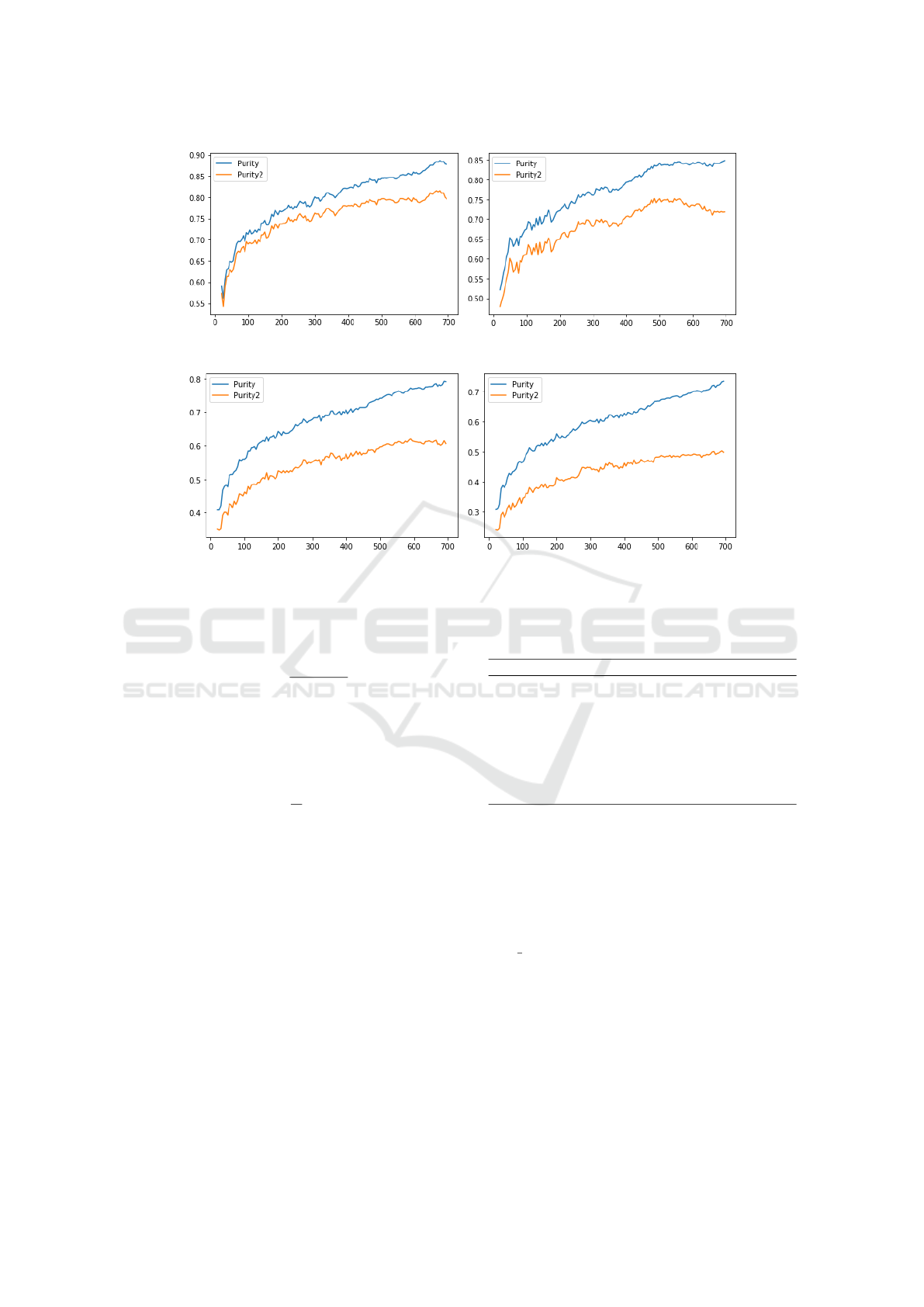
(a) Accuracy STL-10 1000 Images. (b) Accuracy CIFAR-10 1000 Images.

Figure 1: Accuracy comparison in STL-10, Cifar-10, Cifar-100 and Cifar-100/20. We refer to Purity for the full dataset that

contains 1000 images, and to Purity2 for the the dataset without the singleton clusters.

• Recall is the sensitivity:

Recall =

T P

T P + FN

. (3)

• Purity Score which is the measure of purity con-

sidering each cluster with respect to the most fre-

quent class in the cluster (Li and Ding, 2006) We

will refer to this formula as Purity and Accuracy:

Accuracy = Purity =

∑

i=1

max

∩ T

|. (4)

where N is the number of images, k the number of

Cluster, C

the ith cluster, T

is the set of element

of the class j that are present in the cluster C

• Adjusted Rand Index (ADJ) (Hubert and Arabie,

1985)

• Normalised mutual info (NMI) (Strehl and Ghosh,

2002)

3.2 Analysis of Number of Elements per

Group

What this paragraph analyse is the difference between

the number of element for each group. To have a sig-

niﬁcant group of images and at the same a rapid ex-

ecution it has been choosen to randomly take 1000

Table 2: Best Accuracy Results.

Dataset Images per Group Accuracy

STL-10 675 0.887

STL-10

drop

675 0.815

CIFAR-10 695 0.848

CIFAR-10

drop

485 0.751

CIFAR-100/20 690 0.792

CIFAR-100/20

drop

590 0.620

CIFAR-100 695 0.734

CIFAR-100

drop

690 0.502

images for each dataset and analyse their results con-

sidering a number of images for each group from 20

till 700. For the sake of comparison, results are pre-

sented also removing singleton cluster. The aim is

to see in which case are obtained the optimal results

for each dataset. Then next sections present the re-

sult reported in Table 2. In the results, we refer to

Name Dataset

drop

when the dataset has not singleton

clusters because they have been removed by the pro-

posed pipeline.

3.2.1 STL-10

As shown in Figure 1a, the accuracy values obtained

on STL-10 have a growth almost till the end, when the

value starts to slow down again, analysing the number

we see that the maximum value of accuracy consider-

FUB-Clustering: Fully Unsupervised Batch Clustering

159

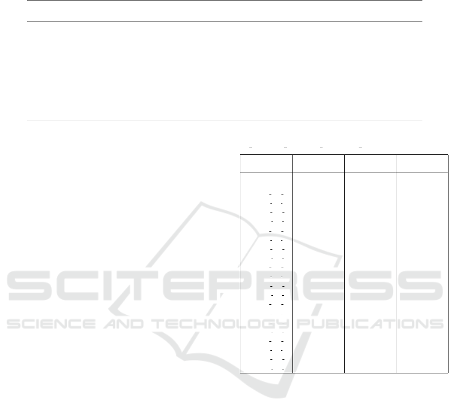
Table 3: Results of Clustering with dataset containing all the images and dataset containing only the cluster with at least 2

elements.

Dataset Max Accuracy Min Accuracy Mean Accuracy Dev Std Accuracy

STL-10 0.890 0.858 0.874 0.008

STL-10

drop

0.816 0.774 0.795 0.013

CIFAR-10 0.836 0.785 0.813 0.011

CIFAR-10

drop

0.752 0.680 0.720 0.014

CIFAR-100/20 0.786 0.731 0.759 0.012

CIFAR-100/20

drop

0.642 0.567 0.605 0.016

CIFAR-100 0.758 0.692 0.730 0.012

CIFAR-100

drop

0.540 0.471 0.500 0.014

ing all cluster and only the cluster that have at least 2

images is when we have 675 elements per group.

3.2.2 Cifar-10

The results in Figure 1b show that the accuracy val-

ues have a growth till the end when we consider every

cluster; when we remove the cluster that have only

one element the growth is approximately till 550 el-

ement per group and the the value starts to go down.

Analysing the number we see that the maximum value

of accuracy considering all cluster is obtained when

there are 695 element per group, and the maximum

value of accuracy considering the cluster that have at

least more than 2 images is 485.

3.2.3 Cifar-100/20

In this Section we will talk about the results on the

dataset CIFAR-100/20. As we can see in Figure 1c

the accuracy values has a growth till the end when

we consider every cluster like it happened in Cifar-

10; when we remove the cluster that have only one

element the growth is approximately till 600 element

per group then the values seems to be stable but lower

than the maximum value. Analysing the number we

see that the maximum value of accuracy considering

all cluster is obtained when there are 690 element per

group, and the maximum value of accuracy consider-

ing the cluster that have at least more than 2 images is

590.

3.2.4 Cifar-100

In this Section we will talk about the results on the

dataset CIFAR-100. As we can see in Figure 1d the

accuracy values has a growth till the end when we

consider every cluster like it happened in Cifar-10 and

Cifar-100/20; but unlike Cifar-10 and Cifar-100/20

the growth is till the end even when we remove the

cluster that have only one element. Analysing the

number we see that the maximum value of accuracy

Table 4: Results of Clustering reduction with the 4 methods:

out max, out avg, max max, max avg iterated 5 times.

Method STL-10 Cifar-10 Cifar-100/20

FUB 0.874±0.008 0.813±0.011 0.759±0.012

FUB

out max 1

0.800±0.035 0.709±0.020 0.667±0.054

FUB

out avg 1

0.803±0.039 0.703±0.018 0.663±0.059

FUB

max max 1

0.846±0.021 0.741±0.019 0.710±0.036

FUB

max avg 1

0.848±0.020 0.743±0.019 0.709±0.038

FUB

out max 2

0.735±0.031 0.639±0.024 0.575±0.039

FUB

out avg 2

0.752±0.038 0.641±0.021 0.565±0.041

FUB

max max 2

0.808±0.019 0.695±0.020 0.636±0.029

FUB

max avg 2

0.808±0.018 0.697±0.018 0.630±0.030

FUB

out max 3

0.691±0.029 0.588±0.022 0.516±0.039

FUB

out avg 3

0.719±0.025 0.597±0.023 0.510±0.035

FUB

max max 3

0.778±0.018 0.659±0.024 0.584±0.026

FUB

max avg 3

0.779±0.019 0.659±0.018 0.572±0.024

FUB

out max 4

0.653±0.030 0.551±0.022 0.478±0.033

FUB

out avg 4

0.701±0.023 0.567±0.025 0.478±0.029

FUB

max max 4

0.757±0.016 0.629±0.024 0.541±0.025

FUB

max avg 4

0.753±0.014 0.624±0.019 0.525±0.020

FUB

out max 5

0.626±0.032 0.521±0.025 0.446±0.030

FUB

out avg 5

0.678±0.026 0.543±0.025 0.458±0.026

FUB

max max 5

0.735±0.020 0.602±0.023 0.507±0.023

FUB

max avg 5

0.734±0.011 0.602±0.021 0.489±0.019

considering all cluster is obtained when there are 695

element per group, and the maximum value of accu-

racy considering the cluster that have at least more

than 2 images is 690.

3.3 Stochastic Batch Clustering and

Clustering Reduction

Each dataset has been divided in random groups of

1000 images; in each group the clustering algorithm

is been executed using as number of images per group

the optimal value that came out from the analysis of

the previous section. In Table 3 is reported a summary

of the results.

As observed earlier, the results may contain sin-

gleton clusters. So to the results it has been applied

the clustering reduction in order to achieve the merg-

ing between singleton clusters and other clusters. Af-

ter the reduction of number of cluster it is expected to

IMPROVE 2023 - 3rd International Conference on Image Processing and Vision Engineering

160

Table 5: Comparations of the results of state of art algorithm

and our algorithm.

Method STL-10 Cifar-10 Cifar-100/20

K-Means

(MacQueen, 1967)

0.192 0.229 0.130

(Ng et al., 2001)

0.159 0.247 0.136

(Franti et al., 2006)

0.332 0.228 0.138

NMF

(Cai et al., 2009)

0.180 0.190 0.118

(Bengio et al., 2006)

0.303 0.314 0.165

SDAE

(Vincent et al., 2010)

0.302 0.297 0.151

DCGAN

(Radford et al., 2015)

0.298 0.315 0.151

DeCNN

(Zeiler et al., 2010)

0.299 0.282 0.133

VAE

(Kingma and Welling, 2013)

0.282 0.291 0.152

JULE

(Yang et al., 2016)

0.277 0.272 0.137

DEC

(Xie et al., 2016)

0.359 0.301 0.185

DAC

(Chang et al., 2017)

0.470 0.522 0.238

DeepCluster

(Caron et al., 2018)

0.334 0.374 0.189

DDC

(Chang et al., 2019)

0.489 0.524 N/A

IIC

(Ji et al., 2019)

0.610 0.617 0.257

DCCM

(Wu et al., 2019)

0.482 0.623 0.327

DSEC

(Chang et al., 2018)

0.482 0.478 0.255

GATCluster

(Niu et al., 2020)

0.583 0.610 0.281

PICA

(Huang et al., 2020)

0.713 0.696 0.337

(Li et al., 2021)

0.850 0.790 0.429

IDFD

(Tao et al., 2021)

0.756 0.815 0.425

SCAN

(Van Gansbeke et al., 2020)

0.809 0.883 0.507

SCAN + RUC

(Park et al., 2021)

0.867 0.903 0.533

SPICE

(Niu et al., 2022)

0.938 0.926 0.538

FUB-Clustering 0.874±0.008 0.81±0.011 0.759±0.012

FUB-Clustering

drop

0.795±0.013 0.72±0.140 0.605±0.016

FUB-Clustering

out max 1

0.800±0.035 0.709±0.020 0.667±0.054

FUB-Clustering

out avg 1

0.803±0.039 0.703±0.018 0.663±0.059

FUB-Clustering

max max 1

0.846±0.021 0.741±0.019 0.710±0.036

FUB-Clustering

max avg 1

0.848±0.020 0.743±0.019 0.709±0.038

observe a lower accuracy because of the merging of

different cluster that not always are 100% accurate so

the errors are also merged; another reason why it is

expected a lower accuracy is that the singleton clus-

ter have accuracy 100% that will not be considered

anymore unless it joins a cluster that is already 100%

accurate. In Table 4 there is a summary of the results

of the clustering reduction. As expected the results

observed have lower accuracy. It is possible to no-

tice also that the methods “out max” and “out avg”

have lower accuracy than “max max” and “max avg”,

however the reason is related to the number of cluster

left, “out max” and “out avg” reduce the number of

cluster so much more than the other two methods.

3.4 Comparison with the State of the

Art

The performance of the FUB-Clustering has been

evaluated on three commonly used dataset: STL-10,

CIFAR-10, CIFAR-100/20. In Table 5 we compare

the results of the different version of FUB and the

result of other state-of-art algorithms. From the re-

sults we can observe that SPICE(Niu et al., 2022) out-

perform FUB in the clustering of the Datasets STL-

10 and Cifar-10. However SPICE require a train-

ing and during the train is known the number of

cluster, instead in FUB the number of cluster is not

known. Our results are still competitive and outper-

form other state-of-art methods. Regarding the Cifar

100/20 Datasets FUB outperforms all the other state-

of-art methods with all the FUB methods, even the

method that drop the singleton clusters.

4 CONCLUSIONS

In this study, we proposed different ways on how to

do clustering using features without prior knowledge

of the number of cluster, K. Our studies have been

performed on images, however this algorithm can be

used with other kinds of data as well. The experimen-

tal results show that FUB-Clustering is competitive

as it outperforms most of the existent state of the art

algorithms on two well known dataset (STL-10 and

Cifar-10) and outperform all the existent state of art

algorithm in the well known dataset Cifar-100/20. It

is worth to highlight that FUB is fully unsupervised,

so it does not have any prior knowledge on the cluster-

ing problem it is applied to (e.g., number of clusters,

kind of input data, dimensionality of the space, etc.).

Other than clustering single images we are also able

to cluster group of images, however if the group of

images is not accurate 100% accurate, we might ob-

tain a some errors in our clustering. Despite FUB-

Clustering is already able to obtain competitive re-

sults, we aim to improve the computational complex-

ity in pursuance of a faster computation.

ACKNOWLEDGEMENTS

This work is partially funded by TIM S.p.A. through

its UniversiTIM granting program

FUB-Clustering: Fully Unsupervised Batch Clustering

161

REFERENCES

Bengio, Y., Lamblin, P., Popovici, D., and Larochelle, H.

(2006). Greedy layer-wise training of deep networks.

Advances in neural information processing systems,

19.

Bishop, C. M. and Nasrabadi, N. M. (2006). Pattern recog-

nition and machine learning, volume 4. Springer.

Cai, D., He, X., Wang, X., Bao, H., and Han, J. (2009).

Locality preserving nonnegative matrix factorization.

In Twenty-ﬁrst international joint conference on arti-

ﬁcial intelligence.

Caron, M., Bojanowski, P., Joulin, A., and Douze, M.

(2018). Deep clustering for unsupervised learning of

visual features. In Proceedings of the European con-

ference on computer vision (ECCV), pages 132–149.

Chang, J., Guo, Y., Wang, L., Meng, G., Xiang, S., and

Pan, C. (2019). Deep discriminative clustering analy-

sis. arXiv preprint arXiv:1905.01681.

Chang, J., Meng, G., Wang, L., Xiang, S., and Pan, C.

(2018). Deep self-evolution clustering. IEEE trans-

actions on pattern analysis and machine intelligence,

42(4):809–823.

Chang, J., Wang, L., Meng, G., Xiang, S., and Pan, C.

(2017). Deep adaptive image clustering. In Proceed-

ings of the IEEE international conference on com-

puter vision, pages 5879–5887.

Coates, A., Ng, A., and Lee, H. (2011). An analy-

sis of single-layer networks in unsupervised feature

learning. In Proceedings of the fourteenth interna-

tional conference on artiﬁcial intelligence and statis-

tics, pages 215–223. JMLR Workshop and Confer-

ence Proceedings.

De la Torre, F. and Kanade, T. (2006). Discriminative clus-

ter analysis. In Proceedings of the 23rd international

conference on Machine learning, pages 241–248.

Franti, P., Virmajoki, O., and Hautamaki, V. (2006). Fast

agglomerative clustering using a k-nearest neighbor

graph. IEEE transactions on pattern analysis and ma-

chine intelligence, 28(11):1875–1881.

Huang, J., Gong, S., and Zhu, X. (2020). Deep semantic

clustering by partition conﬁdence maximisation. In

Proceedings of the IEEE/CVF Conference on Com-

puter Vision and Pattern Recognition, pages 8849–

8858.

Hubert, L. and Arabie, P. (1985). Comparing partitions.

Journal of classiﬁcation, 2(1):193–218.

Ji, X., Henriques, J. F., and Vedaldi, A. (2019). Invariant

information clustering for unsupervised image clas-

siﬁcation and segmentation. In Proceedings of the

IEEE/CVF International Conference on Computer Vi-

sion, pages 9865–9874.

Jiang, Z., Zheng, Y., Tan, H., Tang, B., and Zhou, H.

(2016). Variational deep embedding: An unsuper-

vised and generative approach to clustering. arXiv

preprint arXiv:1611.05148.

Kingma, D. P. and Welling, M. (2013). Auto-encoding vari-

ational bayes. arXiv preprint arXiv:1312.6114.

Krizhevsky, A., Nair, V., and Hinton, G. (2010a). Cifar-10

(canadian institute for advanced research).

Krizhevsky, A., Nair, V., and Hinton, G. (2010b). Cifar-100

(canadian institute for advanced research).

Krizhevsky, A., Sutskever, I., and Hinton, G. E. (2017). Im-

agenet classiﬁcation with deep convolutional neural

networks. Communications of the ACM, 60(6):84–90.

Li, F., Qiao, H., and Zhang, B. (2018). Discrimina-

tively boosted image clustering with fully convolu-

tional auto-encoders. Pattern Recognition, 83:161–

173.

Li, T. and Ding, C. (2006). The relationships among various

nonnegative matrix factorization methods for cluster-

ing. In Sixth International Conference on Data Mining

(ICDM’06), pages 362–371. IEEE.

Li, Y., Hu, P., Liu, Z., Peng, D., Zhou, J. T., and Peng,

X. (2021). Contrastive clustering. In Proceedings of

the AAAI Conference on Artiﬁcial Intelligence, vol-

ume 35, pages 8547–8555.

MacQueen, J. (1967). Classiﬁcation and analysis of mul-

tivariate observations. In 5th Berkeley Symp. Math.

Statist. Probability, pages 281–297.

Ng, A., Jordan, M., and Weiss, Y. (2001). On spectral clus-

tering: Analysis and an algorithm. Advances in neural

information processing systems, 14.

Niu, C., Shan, H., and Wang, G. (2022). Spice: Semantic

pseudo-labeling for image clustering. IEEE Transac-

tions on Image Processing, 31:7264–7278.

Niu, C., Zhang, J., Wang, G., and Liang, J. (2020). Gatclus-

ter: Self-supervised gaussian-attention network for

image clustering. In European Conference on Com-

puter Vision, pages 735–751. Springer.

Ortis, A., Farinella, G. M., D’Amico, V., Addesso, L., Tor-

risi, G., and Battiato, S. (2017). Organizing egocentric

videos of daily living activities. Pattern Recognition,

72:207–218.

Park, S., Han, S., Kim, S., Kim, D., Park, S., Hong, S.,

and Cha, M. (2021). Improving unsupervised image

clustering with robust learning. In Proceedings of the

IEEE/CVF Conference on Computer Vision and Pat-

tern Recognition, pages 12278–12287.

Radford, A., Metz, L., and Chintala, S. (2015). Unsu-

pervised representation learning with deep convolu-

tional generative adversarial networks. arXiv preprint

arXiv:1511.06434.

Strehl, A. and Ghosh, J. (2002). Cluster ensembles—

a knowledge reuse framework for combining multi-

ple partitions. Journal of machine learning research,

3(Dec):583–617.

Tao, Y., Takagi, K., and Nakata, K. (2021). Clustering-

friendly representation learning via instance discrim-

ination and feature decorrelation. arXiv preprint

arXiv:2106.00131.

Van Gansbeke, W., Vandenhende, S., Georgoulis, S., Proes-

mans, M., and Van Gool, L. (2020). Scan: Learning

to classify images without labels. In European confer-

ence on computer vision, pages 268–285. Springer.

Vincent, P., Larochelle, H., Lajoie, I., Bengio, Y., Man-

zagol, P.-A., and Bottou, L. (2010). Stacked denois-

ing autoencoders: Learning useful representations in a

deep network with a local denoising criterion. Journal

of machine learning research, 11(12).

IMPROVE 2023 - 3rd International Conference on Image Processing and Vision Engineering

162

Von Luxburg, U. (2007). A tutorial on spectral clustering.

Statistics and computing, 17(4):395–416.

Wu, J., Long, K., Wang, F., Qian, C., Li, C., Lin, Z.,

and Zha, H. (2019). Deep comprehensive correlation

mining for image clustering. In Proceedings of the

IEEE/CVF International Conference on Computer Vi-

sion, pages 8150–8159.

Xie, J., Girshick, R., and Farhadi, A. (2016). Unsupervised

deep embedding for clustering analysis. In Interna-

tional conference on machine learning, pages 478–

487. PMLR.

Yang, J., Parikh, D., and Batra, D. (2016). Joint unsu-

pervised learning of deep representations and image

clusters. In Proceedings of the IEEE conference on

computer vision and pattern recognition, pages 5147–

5156.

Ye, J., Zhao, Z., and Wu, M. (2007). Discriminative k-

means for clustering. Advances in neural information

processing systems, 20.

Zeiler, M. D., Krishnan, D., Taylor, G. W., and Fergus, R.

(2010). Deconvolutional networks. In 2010 IEEE

Computer Society Conference on computer vision and

pattern recognition, pages 2528–2535. IEEE.

FUB-Clustering: Fully Unsupervised Batch Clustering

163