On the Adjacency Matrix of Spatio-Temporal Neural Network

Architectures for Predicting Traffic

Sebastian Bomher

and Bogdan Ichim

1,2

Faculty of Mathematics and Computer Science, University of Bucharest, Str. Academiei 14, Bucharest, Romania

Simion Stoilow Institute of Mathematics of the Romanian Academy, Str. Calea Grivitei 21, Bucharest, Romania

Keywords: Traffic Models, Neural Network (NN), Graph Convolutional Network (GCN), Long Short-Term Memory

Network (LSTM), Adjacency Matrix.

Abstract: We present in this paper some experiments with the adjacency matrix used as input by three spatio-temporal

neural networks architectures when predicting traffic. The architectures were proposed in (Chen et al., 2022),

(Li et al., 2018) and (Yu et al., 2018). We find that the predictive power of these neural networks is

influenced to a great extent by the inputted adjacency matrix (i.e. the weights associated to the graph of the

available traffic infrastructure). The experiments were made using two newly prepared datasets.

1 INTRODUCTION

Traffic data is very complex and nonlinear. Traffic

forecasting is many times dependent on external

factors such as the time of day, the season of the

year, the climate and current weather, but also on

internal factors such as the available infrastructure,

the number of vehicles on the roads (and their

particular types) or unexpected vehicle crashes. It

plays a crucial role in optimizing traffic flow,

improving traffic speed and efficiency. Moreover, it

is a key element for creating better intelligent

management systems for traffic.

Traffic forecasting is a challenging endeavour.

Its general performance depends on a complex set of

spatio-temporal interdependencies.

In this paper we present several traffic

forecasting experiments for which we use three

spatio-temporal neural network architectures which

were very recently introduced: the GC-LSTM model

(Chen et al., 2022), the DC-RNN model (Li et al.,

2018) and the ST-GCN model (Yu et al., 2018).

These new spatio-temporal neural network

architectures essentially combine some graph

convolutional layers (which are used for processing

the spatial information) with some temporal layers

(used for processing the temporal information). As

an example Long Short-Term Memory Networks

(LSTM), see (Hochreiter et al., 1997), may be used

to build the temporal processing part, but there are

also other choices available. In the experiments

presented here we have focused on the spatial data

used as input for these architectures. For this, we

have developed two new datasets. The data is

provided by the Caltrans Performance Measurement

System (PeMS, 2021). From the raw data a matrix

describing a weighted graph must be prepared as

input, however it is an open question how the

weights should be associated to the available

infrastructure. We have found that the predictive

power of these models is influenced to a great extent

by the way this matrix is prepared.

As a result, the following contributions are made

in this paper:

 We have created two new datasets. These new

datasets contains temporal data for three

different traffic features (flow, speed and

occupancy), as well as spatial data about the

sensors location;

 We have investigated different ways for

computing the weighted graph encoding the

spatial information and the end effect on

prediction. We have tested different parameter

settings from which we select automatically

the best among them for predicting.

 We have also studied to a certain extent the

suitability of the models for predicting the

temporal traffic features.

The code which was used for experiments,

together with the two new prepared datasets, is

available on demand from the authors.

Bomher, S. and Ichim, B.

On the Adjacency Matrix of Spatio-Temporal Neural Network Architectures for Predicting Trafﬁc.

DOI: 10.5220/0011971300003479

In Proceedings of the 9th International Conference on Vehicle Technology and Intelligent Transport Systems (VEHITS 2023), pages 321-328

ISBN: 978-989-758-652-1; ISSN: 2184-495X

 2023 by SCITEPRESS – Science and Technology Publications, Lda. Under CC license (CC BY-NC-ND 4.0)

321

2 RELATED WORK

Scientists have been and are still looking for ways to

optimize traffic flow, improve traffic speed and

create better intelligent management systems for

traffic. Therefore, forecasting traffic is currently a

major research topic. Various authors have

investigated many approaches to the problem of

traffic forecasting. Nowadays, as a result of the rapid

development in the field of deep learning (Moravčík

et al., 2016), (Silver et al., 2016), (Silver et al.,

2017), certain new neural networks architectures

have received particular attention. Many times they

deliver the top results when compared with other

models.

Frequently the old approaches ignore completely

the spatial features particular to the traffic, focusing

only on temporal features (as for example flow and

speed). These models are operating like processing

the temporal traffic data is not at all restricted by the

available spatial framework. Nonetheless, it is clear

that only by using both the temporal information and

the spatial information performant traffic forecasting

might be achieved.

As a result of the given topology of the existing

roads networks the spatial traffic information is

intrinsically belonging to the graphs area of

research. In the last years a more general version of

the well-known Convolutional Neural Networks

(CNN) architecture was developed for usage given

that data may be linked to graph domains. It is called

Graph Convolutional Network (GCN) and

essentially uses as input a matrix describing a

weighted graph. For more information about GCN

and their development we point the reader to (Bruna

et al., 2014), (Henaff et al., 2015), (Atwood and

Towsley, 2016), (Niepert et al., 2016), (Kipf and

Welling, 2017) and (Hechtlinger et al., 2017). Note

that the GCN architecture was used by many authors

since its introduction for various applications and

has delivered superior performance.

Recently several authors have developed various

GCN architectures that may be used for forecasting

traffic, being motivated by the ability of GCN to

process data linked to graph domains. In (Li et al.,

2018) the authors propose a model computing

random walks on graphs. This was one of the first

attempts for making the spatial features useful. This

work was followed quite quickly by several related

papers, for example (Yu et al., 2018), (Zhao et al.,

2020), (Zhang et al., 2020), (Li and Zhu, 2021) and

(Chen et al., 2022). The authors investigate how

traffic forecasting may be improved by using various

architectures of spatio-temporal neural networks. In

general, they only use a certain fixed matrix in order

to describe the associated weighted graph.

Continuing this line of research, we perform

several experiments in order to see if the content of

this input matrix does play an important role for the

performance obtained by some particular spatio-

temporal neural network architecture and which way

of computing its entries (i.e. the weights associated

to the graph) does provide superior performance.

3 METHODOLOGY

3.1 Problem Statement

The aim of this paper is to study the influence that

the knowledge about the sensors spatial position on

the roads and the way it is further processed has on

predicting traffic features like flow, speed and

occupancy. All these are simultaneously available in

the data stored by the Caltrans Performance

Measurement System (PeMS, 2021).

Denote by 𝑆 be the number of sensors and by 𝑁

the number of time steps in a certain dataset. The

spatial information about the sensors will be

contained in a matrix 𝐴∈ℝ



which it is called the

adjacency matrix and contains certain weights 𝑎



∈



0,1



. Remark that there exists no standard

procedure for inputting the weights 𝑎



. We note that

they should be close to be 0 if there is a bad roadway

network between the two linked sensors 𝑖 and 𝑗, and

to be close to 1 if there a good roadway network

between them.

Further, if 𝐾 traffic features (like flow, speed

and occupancy) are considered, then we get 𝐾x𝑆

time-series which are gathered by the traffic sensors.

Assume they are stored in a feature matrix 𝐵∈

ℝ



. Then, the vector 𝐵



∈ℝ



contains the

values collected for all available traffic features and

by all sensors at a certain time 𝑡.

Let 𝑇 be a number of time steps. For given

adjacency matrix 𝐴 and feature matrix 𝐵, the

general problem of spatio-temporal traffic

forecasting over the time horizon 𝑇 is the problem of

learning a model 𝑀 (i.e. a function) such that

𝐵



≈𝑀𝐴;

(

𝐵



,…,𝐵



,𝐵



)

.

In this paper we focus our attention on the

adjacency matrix 𝐴. We investigate different ways

for choosing 𝑎



in order to construct the adjacency

matrix 𝐴 and observe their influence on the model

performance in several computational experiments.

VEHITS 2023 - 9th International Conference on Vehicle Technology and Intelligent Transport Systems

322

3.2 The Architecture of the

Spatio-Temporal Neural Networks

For the experiments presented in this paper we use

three spatio-temporal neural network architectures:

the GC-LSTM model (Chen et al., 2022), the DC-

RNN model (Li et al., 2018) and the ST-GCN model

(Yu et al., 2018).

The architecture of the GC-LSTM model (Chen

et al., 2022) is illustrated in Figure 1.

Figure 1: The architecture of the GC-LSTM model. The

𝐾x𝑆 time series collected by the traffic stations are used as

input.

According to (Chen et al., 2022) the GC-LSTM

model consists of two distinct parts: the GCN part

and the LSTM part. In order to apprehend the spatial

relation between traffic stations the GCN part is

used first. The graph convoluted data is expanded

next with the temporal data contained in the 𝐾x𝑆

time series. Then the time-series (now augmented

with a graph convolution containing spatial features)

are loaded in the LSTM part. The LSTM part keeps

track of previous information as well.

The architecture of the DC-RNN model (Li et

al., 2018) is very similar to the above architecture.

The main difference is that instead of LSTM, the

authors use Gated Recurrent Units (GRU). The same

idea is also used by (Zhao et al., 2020). According to

(Chung et al., 2014), the basic operating principles

of both the GRU and LSTM are approximately the

same. As can be also observed from the experiments

presented in this paper they deliver in practice

similar performance for various tasks, so we have

not noticed significant differences between them.

According to (Yu et al., 2018) the ST-GCN

model consists of two Spatio-Temporal Convolution

blocks (ST-Conv blocks) after which an extra

temporal convolution layer with a fully-connected

layer as the output layer is added. Each ST-Conv

block is made of two Temporal Gated Convolution

layers with one Spatial Graph Convolution layer

sandwiched between them. Each Temporal Gated

Convolution contains a Gated Linear Unit (GLU)

with a one-dimensional convolution. Figure 2

illustrates this architecture.

Figure 2: The architecture of the ST-GCN model (left) and

the architecture of a single ST-Conv block (right).

In summary, all three architectures used in the

experiments are universal frameworks for capturing

complex spatial and temporal characteristics.

3.3 Dataset

For performing experiments we have processed two

new datasets using traffic information which was

gathered from the city of Los Angeles, California.

The data is aggregated from sensors positioned on

the various roads within the state of California and it

is stored and publically available in the Caltrans

Performance Measurement System (PeMS, 2021), a

public web platform where users can analyse and

export traffic information. In particular the website

offers multiple sectors of the city of Los Angeles.

For preparing the datasets sector seven was chosen.

This sector contains a total of 4904 unique traffic

stations each having its own identifier. However, the

raw data available from PeMS platform contains

many observations for which the values of the traffic

features are simply not available. A first important

step was to check the correctitude of the available

information. To this scope a python script passes

through each row of data and checks if the

corresponding traffic station contains information

about speed, occupancy and flow. If all three are

present then it is considered a good sensor and it is

saved. After this step from 4904 sensors only 2789

are left. A second important step in preparing the

datasets was to select traffic stations which are

relatively close together (so that we may assume that

On the Adjacency Matrix of Spatio-Temporal Neural Network Architectures for Predicting Trafﬁc

323

the corresponding traffic values are related). This

was done by plotting on a map the sensors and then

hand-picking them.

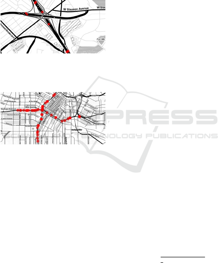
The first dataset, called in the following small,

contains 8 hand-picked sensors in an intersection.

Their location is shown in Figure 3.

Figure 3: Map of the hand-picked sensors for the small

dataset.

The second dataset, called in the following

medium, contains 50 hand-picked sensors around an

intersection, as shown in Figure 4.

Figure 4: Map of the hand-picked sensors for the medium

dataset.

For the selected sensors, the two datasets contain

complete temporal data for the most important

traffic features available in the PeMS platform, i.e.

flow, speed and occupancy. Both datasets enclose

the time interval from the 1

of July to the 31

July 2021. Remarking that the heaviest congestion

happens during the week days and in order to find

better insight of the traffic during the most critical

periods only the 22 weekdays of July 2021 are

selected for further use. Measurements on each

sensor are done every 5 minutes. There are 288

observations for every day. In total both datasets

contain 6336 observations for each sensor.

The PeMS platform also offers an extra metadata

file which provides additional information for each

individual traffic station. From the data available for

each sensor the latitude and longitude numbers are

further used for computing the spatial information

needed for the experiments.

3.4 Technical Implementation

Python is the most popular programming language

used for artificial intelligence, data science or

machine learning projects in general. It is probably

the best choice for performing experiments similar

with those presented in this paper.

After the data is downloaded from the PeMS

platform it requires further processing. For this

scope the libraries Pandas (Pandas, 2016) and

NumPy (Harris et al., 2020) have been used.

Further, for the implementation of the spatio-

temporal neural network models we have used the

Python versions of the state of the art libraries

Tensorflow, Keras and Torch. Tensorflow (Google

Brain, 2016) is a library developed by Google for

implementing machine learning applications. On top

of Tensorflow, another very popular package, named

Keras (Chollet, 2015), has been built. It contains

various implementations of machine learning

algorithms and together with the StellarGraph

library (CSIRO's Data61, 2018) was used for the

experiments done in (Ichim and Iordache, 2022). For

most machine learning projects Keras is the standard

choice. Torch (Paszke et al., 2019) is another well-

known library based on TensorFlow which contains

a collection of advanced tools for machine learning.

It is harder to use as Keras since the training step

needs to be manually implemented, however with

more flexibility, it has more to offer. It was our

choice for the experiments done below.

4 EXPERIMENTS

4.1 Performance Metrics

There are multiple ways to compute the performance

of a certain model. For our experiments we have

chosen five standard loss functions that compute the

distance between the actual, as measured value of a

feature y

, and the value predicted by the model for

the same feature. Let us suppose that the dataset

used for testing contains 𝑁 observations (samples)

of the shape

(

𝑥



,𝑦



)

and 𝑚 is the model for which

the performance is computed. Denote by 𝑚

(

𝑥



)

the

model prediction for 𝑦



and let 𝑦



 be the arithmetic

mean of 𝑦



. Then we have:

 Root Mean Squared Error (RMSE):

𝑅𝑀𝑆𝐸

(

𝑚

)









(

𝑦



−𝑚(𝑥



)







;

VEHITS 2023 - 9th International Conference on Vehicle Technology and Intelligent Transport Systems

324

 Mean Absolute Percentage Error (MAPE):

𝑀𝐴𝑃𝐸(𝑚)=

100

𝑁



𝑦



−𝑚

(

𝑥



)

𝑚

(

𝑥



)

;





 Mean Absolute Error (MAE):

𝑀𝐴𝐸

(

𝑚

)







𝑦



−𝑚(𝑥



)





;

 Mean Squared Error (MSE):

𝑀𝑆𝐸

(

𝑚

)







(

𝑦



−𝑚(𝑥



)







;

 The Coefficient of Determination (R

𝑅



(

𝑚

)

=1−



(

𝑦



−𝑚(𝑥



)







∑(

𝑦



−𝑦





)







More specifically, the first four metrics measure

the loss in the model prediction. Their interpretation

is the following: a small calculated value means a

better model at making predictions. The coefficient

of determination measures the (abstract) ability to

provide good predictions by comparing a given

model with the trivial model. It is always less than 1

by definition and it is 0 for the trivial model. A

coefficient of determination close to 1 indicates a

model which is significantly better than the trivial

model.

In the tables below we compute the final RMSE

as an arithmetic average over time of the RMSE

computed for all sensors at a single time moment.

Since for any positive values 𝑎



we have

∑



𝑎







𝑁





𝑁

𝑎







it follows that the final RMSE reported is smaller

than the square root of the final MSE reported.

4.2 Setup for Experiments

The neural network architectures which were used in

experiments use graphs as inputs and for this reason

the corresponding adjacency matrices need to be

constructed. Since our experiments have focused on

the influence that the input adjacency matrix plays

on the final performance we have considered the

following setups:

 Two different datasets. They essentially

determine the number of vertices in the

graph

o Small – 8 vertices;

o Medium – 50 vertices;

 Three possible ways for establishing when

there exists a edge between two vertices

o Complete – the graph has an edge

between every two vertices;

o Manual – using the map, the

vertices are manually connected;

o LR – we experimentally try to

use standard linear regression in

order to connect the vertices;

 Two distinct methods for computing the

distances between two vertices

o Geodesic – using the latitude and

longitude data for each sensor, the

geodesic distance between two

sensors is computed;

o OSRM – the shortest paths in the

road network is computed using

data from (OSRM, 2023).

Further, the weights associated to the edges need

to be computed. For this we use the following

formula

𝑤



=exp−

𝑑





𝜎



if 𝑖𝑗 and exp−

𝑑





𝜎



𝜖,

which was proposed in (Yu et al., 2018). Here 𝑤



represents the weight of adjacency matrix

corresponding to the distance 𝑑



between the

vertices 𝑖 and 𝑗 computed above. The two tuning

hyperparameters 𝜖 and 𝜎 introduced in the formula

are thresholds used in order control the sparsity and

the distribution of the graph’s edges. A grid search is

performed for tuning these hyperparameters. After

this the best settings are selected automatically and

they are used further for making predictions. The

values given for the two parameters in the grid

search are:

𝜎∈



1,3,5, 10



and 𝜖∈



0.1,0.3,0.5,0.7



4.3 Results of the Experiments

The performance of a GC-LSTM model (Chen et al.,

2022) is compared below with the performance of a

DC-RNN model (Li et al., 2018) and with the

performance of a ST-GCN model (Yu et al., 2018).

On the Adjacency Matrix of Spatio-Temporal Neural Network Architectures for Predicting Trafﬁc

325

This allows us to see the effects that the various

changes made to the input adjacency matrix have on

the combined spatio-temporal prediction potential of

the models.

The final results of our experiments are

contained in Table 1 for the small dataset and in

Table 2 for the medium dataset. We have marked

with bold the best predictions made by each of the 3

models for 3 ways of constructing the edges

(complete, manual and linear regression) and for 2

different ways for computing the associated

distances (geodesic and OSRM). In our experiments

we have predicted the speed, however there is no

restriction in repeating the experiment for

forecasting other temporal traffic features (like flow

or occupancy). Overall the ST-GCN model has

provided the best performance in these experiments.

Table 1: Experimental Results on Small Dataset.

Model Edges Distances

Metric

RMSE MAPE MAE MSE R

GC-LSTM

Complete

Geodesic 12.3186 0.3245 9.3377 230.1765 -0.0939

OSRM 2.7649 0.0481 2.0921 11.0771 0.9474

Manual

Geodesic 4.9872 0.0697 3.2098 38.4739 0.8172

OSRM 4.8829 0.0703 3.2358 35.5279 0.8312

Geodesic 9.3054 0.1732 7.2134 146.5231 0.3037

OSRM 8.6787 0.1864 7.0297 128.3809 0.3899

DC-RNN

Complete

Geodesic 13.0717 0.3477 9.8091 261.9677 -0.2451

OSRM 3.0782 0.0536 2.2542 14.5672 0.9308

Manual

Geodesic 4.7836 0.0682 3.0916 34.6671 0.8352

OSRM 4.7451 0.0676 3.0761 34.7506 0.8349

Geodesic 10.2666 0.1901 7.5919 178.4229 0.1521

OSRM 9.2368 0.1769 6.9151 144.4572 0.3135

ST-GCN

Complete

Geodesic 2.5141 0.0407 1.7378 8.0861 0.9616

OSRM 2.5936 0.0413 1.8111 8.7246 0.9585

Manual

Geodesic 2.9377 0.0458 2.0689 10.4536 0.9503

OSRM 2.5497 0.0409 1.7913 8.2218 0.9609

Geodesic 2.5839 0.0417 1.8082 8.5089 0.9596

OSRM 3.2609 0.0599 2.2025 12.4608 0.9408

Table 2: Experimental Results on Medium Dataset.

Model Edges Distances

Metric

RMSE MAPE MAE MSE R

GC-LSTM

Complete

Geodesic 9.2198 0.2202 7.1484 129.7562 0.1016

OSRM 3.1074 0.0505 2.4401 12.1576 0.9158

Manual

Geodesic 8.4881 0.1997 5.6513 111.5111 0.2279

OSRM 8.2374 0.1946 5.6716 104.5321 0.2763

Geodesic 8.3699 0.1784 5.8521 106.3525 0.2637

OSRM 8.2734 0.1741 5.8059 103.7811 0.2815

DC-RNN

Complete

Geodesic 9.1336 0.2023 6.9403 128.6674 0.1092

OSRM 5.1074 0.1006 3.9828 35.7923 0.7522

Manual

Geodesic 8.4088 0.1971 5.5235 108.7543 0.2471

OSRM 8.4106 0.2001 5.6183 110.1817 0.2372

Geodesic 8.2222 0.1742 5.7521 102.5802 0.2898

OSRM 8.2052 0.1755 5.7703 101.7261 0.2957

ST-GCN

Complete

Geodesic 2.2045 0.0291 1.4141 5.6623 0.9608

OSRM 3.0271 0.0331 1.6851 9.8946 0.9315

Manual

Geodesic 2.9934 0.0351 1.7708 9.7289 0.9326

OSRM 2.1745 0.0303 1.3569 5.8831 0.9593

Geodesic 3.1474 0.0303 1.5051 10.6289 0.9264

OSRM 2.1291 0.0282 1.3691 5.2089 0.9639

VEHITS 2023 - 9th International Conference on Vehicle Technology and Intelligent Transport Systems

326

4.4 Interpretation of the Results

The scope of the following visualizations is to

provide a better understanding of our results. We

have chosen two particular sensors (one for the

small and one for the medium dataset) and the

predictions made for traffic speed by all three

models for both datasets on the corresponding test

sets are presented in the Figures 5 and 6.

Figure 5: GC-LSTM, DC-RNN and ST-GCN speed

predictions on one sensor of the small dataset.

Figure 6: GC-LSTM, DC-RNN and ST-GCN speed

predictions on one sensor of the medium dataset.

Analysing the performance obtained (as

presented in Tables 1 and 2), we can see that:

 By using data from (OSRM, 2023) for

computing distances (i.e. the associated

weight of the adjacency matrix) we get better

performance in general (independent of the

model). On the small dataset there exists one

experimental setup where the best

performance is obtained with the distances

computed as geodesic distances, however the

difference is not significant;

 In general the complete graph appears to

provide the best performance, but only when

combined with the OSRM computed

distances. This was really a surprise for us,

since it provides significantly better

performance than even the manually

constructed graphs. On the medium dataset

there exists one experimental setup where the

best performance is obtained with our

experimental variation of the linear regression

algorithm, however the difference is not

significant.

5 CONCLUSIONS AND FUTURE

WORK

We present in this paper some experiments with the

adjacency matrix used as input by three spatio-

temporal neural networks architectures when

predicting traffic. For the experiments the following

architectures were used: the GC-LSTM model (Chen

et al., 2022), the DC-RNN model (Li et al., 2018)

and the ST-GCN model (Yu et al., 2018). For each

architecture we have considered 12 experimental

setups, which were given by variations of the input

adjacency matrix. We have found that, in almost all

cases, the best performance is obtained when

combining the complete graph with OSRM

computed distances. In the two cases were the values

obtained for R

were negative (see Table 1) the

model has delivered worse performance than the

trivial model, which shows the importance of the

method used for computing the distances. However,

one should note that there are significant limitations

to this approach, since the complexity of the

complete graph increases quadratically with the

number of vertices in the graph and the graphs

considered are not really big.

In the future we plan to make more experiments

with both the spatial data (represented in the

adjacency matrix), as well as with the temporal

On the Adjacency Matrix of Spatio-Temporal Neural Network Architectures for Predicting Trafﬁc

327

traffic data. It is quite clear that the way the spatial

information is pre-processed plays an important role

for improving the overall performance. Therefore we

intend to search for better ways of processing it,

aiming in particular for a sparse representation. We

also intend to investigate more complex dataset, like

for example the dataset introduced in (Mon et al.,

2022).

REFERENCES

Atwood, J., Towsley, D. (2016). Diffusion-convolutional

neural networks. In NIPS'16, Proceedings of the 30th

International Conference on Neural Information

Processing Systems, 2001 – 2009.

Bruna, J., Zaremba, W., Szlam, A., LeCun, Y. (2014).

Spectral Networks and Locally Connected Networks

on Graphs. In ICLR 2014, Proceedings of the 2th

International Conference on Learning

Representations, pages 1 – 14.

Chen, J., Wang, X., Xu, X. (2022). GC-LSTM: graph

convolution embedded LSTM for dynamic network

link prediction. Applied Intelligence 52, pages 7513 –

7528.

Chollet, F., & others (2015). Keras. Available online at:

https://github.com/fchollet/keras.

Chung, J., Gulcehre, C., Cho, K., Bengio, Y. (2014).

Empirical Evaluation of Gated Recurrent Neural

Networks on Sequence Modeling. Presented in NIPS

2014, Deep Learning and Representation Learning

Workshop. Preprint arXiv: 1412.3555.

CSIRO's Data61 (2018). StellarGraph Machine Learning

Library. Online at https://stellargraph.readthedocs.io/.

Google Brain (2016). TensorFlow: A system for large-

scale machine learning. In OSDI'16, Proceedings of

the 12th USENIX conference on Operating Systems

Design and Implementation, pages 265 – 283.

Harris, R., Millman, J., van der Walt, J. et al. (2020).

Array programming with NumPy. Nature 585, pages

357 – 362.

Hechtlinger, Y., Chakravarti, P., Qin, J. (2017). A

generalization of convolutional neural networks to

graph-structured data. Preprint arXiv: 1704.08165.

Henaff, M., Bruna, J., LeCun, Y. (2015). Deep

convolutional networks on graph-structured data.

Preprint arXiv:1506.05163.

Hochreiter, S., Schmidhuber, J. (1997). Long short-term

memory. Neural Computation 9, pages 1735 – 1780.

Ichim, B., Iordache, F. (2022). Predicting Multiple Traffic

Features using a Spatio-Temporal Neural Network

Architecture. In VEHITS 2022, Proceedings of the 8th

International Conference on Vehicle Technology and

Intelligent Transport Systems, pages 331 – 337.

Kipf, T., Welling, M. (2017). Semi-Supervised

Classification with Graph Convolutional Networks. In

ICLR 2017, Proceedings of the 6th International

Conference on Learning Representations, pages 1 –

14.

Li, Y., Yu, R., Shahabi, C., Liu, Y. (2018). Diffusion

Convolutional Recurrent Neural Network: Data-

Driven Traffic Forecasting. In ICLR 2018,

Proceedings of the 6th International Conference on

Learning Representations, pages 1 – 16.

Li, M., Zhu, Z. (2021). Spatial-temporal fusion graph

neural networks for traffic flow forecasting. In

Proceedings of the Thirty-Five AAAI Conference on

Artificial Intelligence, 4189 – 4196.

Mon, E., Ochiai, H., Komolkiti, P., Aswakul, C. (2022).

Real-world sensor dataset for city inbound-outbound

critical intersection analysis. Scientific Data 9, article

number 357.

Moravčík, M., Schmid, M., Burch, N., Lisý, V., Morrill,

D., Bard, N., Davis, T., Waugh, K., Johanson, M.,

Bowling, M. (2017). Deepstack: Expert-level artificial

intelligence in heads-up no-limit poker. Science 356,

pages 508 – 513.

Niepert, M., Ahmed, M., Kutzkov, K. (2016). Learning

convolutional neural networks for graphs. In ICML

2016, Proceedings of the 33rd International

Conference on Machine Learning, pages 2014 – 2023.

Pandas (2020). Available at: https://pandas.pydata.org/.

Paszke, A., Gross, S., Massa, F., Lerer, A., Bradbury, J.,

Chanan, G., et al. (2019). PyTorch: An Imperative

Style, High-Performance Deep Learning Library.

Advances in Neural Information Processing Systems

32, pages 8024 – 8035.

PeMS, Caltrans Performance Measurement System

(2021). Data available at https://pems.dot.ca.gov/.

OSRM, Open Source Routing Machine (2023). Data

available at http://project-osrm.org/.

Silver, D. et al. (2016). Mastering the game of go with

deep neural networks and tree search. Nature 529,

pages 484 – 489.

Silver, D. et al. (2017). Mastering the game of go without

human knowledge. Nature 550, pages 354 – 359.

Yu, B., Yin, H., Zhu, Z. (2018). Spatio-Temporal Graph

Convolutional Networks: A Deep Learning

Framework for Traffic Forecasting. In Proceedings of

the Twenty-Seventh International Joint Conference on

Artificial Intelligence, IJCAI-ECAI-2018, pages 3634

– 3640.

Zhang, Q., Chang, J., Meng, G., Xiang, S., Pan, C. (2020).

Spatio-Temporal Graph Structure Learning for Traffic

Forecasting. In Proceedings of the Thirty-Fourth AAAI

Conference on Artificial Intelligence, 1177 – 1185.

Zhao, L., Song, Y., Zhang, C., Liu, Y., Wang, P., Lin, T.,

Deng, M., Li H. (2020). T-GCN: A Temporal Graph

Convolutional Network for Traffic Prediction. IEEE

Transactions on Intelligent Transportation Systems

21, pages 3848 – 3858.

VEHITS 2023 - 9th International Conference on Vehicle Technology and Intelligent Transport Systems

328