RePAD2: Real-Time Lightweight Adaptive Anomaly Detection for

Open-Ended Time Series

Ming-Chang Lee

1 a

and Jia-Chun Lin

2 b

Department of Computer science, Electrical engineering and Mathematical Sciences,

Høgskulen p

a Vestlandet (HVL), Bergen, Norway

Department of Information Security and Communication Technology,

Norwegian University of Science and Technology (NTNU), Gjøvik, Norway

Keywords:

Time Series, Open-Ended Time Series, Univariate Time Series, Real-Time Anomaly Detection, LSTM,

Adaptive Detection Threshold, Sliding Window.

Abstract:

An open-ended time series refers to a series of data points indexed in time order without an end. Such a

time series can be found everywhere due to the prevalence of Internet of Things. Providing lightweight and

real-time anomaly detection for open-ended time series is highly desirable to industry and organizations since

it allows immediate response and avoids potential ﬁnancial loss. In the last few years, several real-time time

series anomaly detection approaches have been introduced. However, they might exhaust system resources

when they are applied to open-ended time series for a long time. To address this issue, in this paper we

propose RePAD2, a real-time lightweight adaptive anomaly detection approach for open-ended time series

by improving its predecessor RePAD, which is one of the state-of-the-art anomaly detection approaches. We

conducted a series of experiments to compare RePAD2 with RePAD and another similar detection approach

based on real-world time series datasets, and demonstrated that RePAD2 can address the mentioned resource

exhaustion issue while offering comparable detection accuracy and slightly less time consumption.

1 INTRODUCTION

A time series refers to a series of data points or obser-

vations obtained through repeated measurements over

time (Ahmed et al., 2016). In the real world, many

time series are continuously observed and collected.

They are called open-ended time series in this paper

because they do not have an end point. Such time se-

ries can be found everywhere due to the prevalence of

the Internet of Things. Examples include CO2 lev-

els measured by air quality monitors, human heart

rates or blood pressure measured by medical IoT de-

vices, electricity consumption by smart meters, hu-

midity levels by smart agriculture IoT devices, water

ﬂow and saturation levels by smart ocean monitoring

systems, etc.

Anomaly detection refers to a data analysis task

that detects anomalous or abnormal data from a given

dataset (Ahmed et al., 2016). An anomaly is de-

ﬁned as “an observation which deviates so much

from other observations as to arouse suspicions that it

https://orcid.org/0000-0003-2484-4366

https://orcid.org/0000-0003-3374-8536

was generated by a different mechanism” (Hawkins,

1980). Anomaly detection has been widely applied in

many application domains such as intrusion detection,

fraud detection, industrial damage, sensor network,

healthcare, etc. (Hochenbaum et al., 2017; Aggarwal

and Yu, 2008; Xu and Shelton, 2010; Fisher et al.,

2016; Wu et al., 2018; Staudemeyer, 2015; Bontemps

et al., 2016). We believe that providing real-time and

lightweight anomaly detection for open-ended time

series is highly desirable to industry and organizations

since it enables immediate response, allows appropri-

ate countermeasure to be promptly taken, and avoids

the occurrence of catastrophic failures/events.

During the past few years, several real-time and

lightweight anomaly detection approaches have been

introduced for time series, such as RePAD (Lee et al.,

2020b) and its two successors ReRe (Lee et al.,

2020a) and SALAD (Lee et al., 2021b). However,

RePAD suffers from a resource exhaustion issue due

to its design in determining its adaptive detection

threshold. More speciﬁcally, the adaptive detection

threshold will be periodically recalculated based on

all previously derived average absolute relative error

208

Lee, M. and Lin, J.

RePAD2: Real-Time Lightweight Adaptive Anomaly Detection for Open-Ended Time Series.

DOI: 10.5220/0011981700003482

In Proceedings of the 8th International Conference on Internet of Things, Big Data and Security (IoTBDS 2023), pages 208-217

ISBN: 978-989-758-643-9; ISSN: 2184-4976

 2023 by SCITEPRESS – Science and Technology Publications, Lda. Under CC license (CC BY-NC-ND 4.0)

(AARE) values. Hence, when RePAD works on an

open-ended time series for a long time, it will eventu-

ally exhaust the system resources. The same situation

will also happen to ReRe and SALAD since they in-

herit the threshold design from RePAD.

To address the above-mentioned resource exhaus-

tion issue, in this paper, we propose RePAD2 by im-

proving RePAD in designing the adaptive detection

threshold. Instead of relying on all historical AARE

values to calculate the detection threshold, RePAD2

only calculates the detection threshold based on a

ﬁxed number of recently derived AARE values. In

other words, we employ the concept of sliding win-

dow to redesign the threshold. However, it is unclear

how different sliding window sizes impact the detec-

tion accuracy and time consumption of RePAD2.

To demonstrate the performance of RePAD2, we

conducted a series of experiments based on real-world

time series data from the Numenta Anomaly Bench-

mark (NAB, 2015) and compared RePAD2 with an-

other two state-of-the-art real-time anomaly detec-

tion approaches. The experiment results show that

RePAD2 with a sufﬁciently long sliding window can

provide comparable prediction accuracy and slightly

less time consumption.

The rest of the paper is organized as follows: Sec-

tion 2 describes related work. Section 3 describes

RePAD. In Section 4, we present how RePAD2 im-

proves RePAD. Section 5 presents and discusses the

experiments and the corresponding results. In Section

6, we conclude this paper and outline future work.

2 RELATED WORK

During the past decades, a number of anomaly detec-

tion approaches have been introduced, and they can

be divided into two categories: Statistical learning ap-

proaches and machine-learning approaches.

Statistical learning approaches work by creating a

statistical model for a set of normal data and then use

the model to determine if a data point ﬁts this model

or not. If the data point has a low probability to be

generated from the model, it is considered anomalous.

For examples, AnomalyDetectionTs and Anomaly-

DetectionVec are statistical learning approaches pro-

posed by Twitter (Twitter, 2015). AnomalyDetec-

tionTs was designed to detect statistically signiﬁcant

anomalies in a given time series. On the other hand,

AnomalyDetectionVec was designed to detect statis-

tically signiﬁcant anomalies in a given vector of ob-

servations without timestamp information. However,

both approaches are parameter sensitive because they

require human experts to set appropriate values to

their parameters in order to achieve good detection

performance.

Luminol (LinkedIn, 2018) is another statistical-

based anomaly detection approach proposed by

LinkedIn to identify anomalies in real user monitor-

ing data. Given a time series, Luminol calculates an

anomaly score for each data point. If a data point has

a high score, it indicates that this data point is likely

to be anomalous. However, human experts still need

to further determine which data points are anomalies

based on their domain knowledge and experiences.

Siffer et al. (Siffer et al., 2017) introduced a time

series anomaly detection approach based on Extreme

Value Theory. This approach makes no assumption on

the distribution of time series and requires no thresh-

old manually set by humans. However, this approach

needs a long period to do necessary calibration before

conducting anomaly detection.

On the other hand, most machine learning-based

anomaly detection approaches require either domain

knowledge or human intervention. For instances, Ya-

hoo proposed EGADS (Laptev et al., 2015) to de-

tect anomalies on time series based on a collection

of anomaly detection and forecasting models. How-

ever, EGADS requires to model the target time series

so as to predict a data value later used by its anomaly

detection module and its altering module. Lavin and

Ahmad (Lavin and Ahmad, 2015) introduced Hierar-

chical Temporal Memory to capture pattern changes

in time series. However, this approach requires 15%

of its training dataset to be non-anomalous for train-

ing its neural network.

Greenhouse (Lee et al., 2018) is an anomaly

detection algorithm for time series based on Long

Short-Term Memory (LSTM for short) (Hochreiter

and Schmidhuber, 1997), which is an neural network

designed to learn long short-term dependencies and

model temporal sequences. Greenhouse requires all

its training dataset to be non-anomalous. During the

training phase, Greenhouse adopts a Look-Back and

Predict-Forward strategy to detect anomalies. For a

given time point, a window of most recently observed

data point values of length b is used as a Look-Back

period to predict a subsequent window of data point

values of length f. This feature enables Greenhouse to

adapt to pattern changes in the training data. How-

ever, Greenhouse requires an ofﬂine training phase

to train its LSTM model, and its detection threshold

must be speciﬁed by human experts.

RePAD (Lee et al., 2020b) is one of the state-of-

the-art real-time and lightweight time series anomaly

detection approaches, and it is also based on LSTM

and the Look-Back and Predict-Forward strategy.

However, unlike Greenhouse, RePAD does not need

RePAD2: Real-Time Lightweight Adaptive Anomaly Detection for Open-Ended Time Series

209

an ofﬂine training phase. RePAD utilizes a simple

LSTM network (with one hidden layer and ten hidden

units) trained with short-term historical data points

to predict upcoming data points, and then decides if

each data point is anomalous based on a dynamic de-

tection threshold that can adapt to pattern changes in

the target time series. However, RePAD needs to re-

calculate its detection threshold based on all histori-

cal AARE values at every time point (except the ﬁrst

few time points). Hence, when RePAD works on an

open-ended time series, it might eventually exhaust

the underlying system resources.

ReRe (Lee et al., 2020a) is an enhanced real-time

time series anomaly detection based on RePAD, and

it was designed to keep a high true positive rate and a

low false positive rate. It utilizes two LSTM models

to jointly detect anomalous data points. One of the

LSTM models works exactly as RePAD, whereas the

other LSTM model works similar to RePAD but with

a stricter detection threshold.

3 RePAD

Before introducing RePAD2, let us understand how

RePAD works. Figure 1 illustrates the algorithm of

RePAD (Lee et al., 2020b). RePAD uses short-term

historical data points to predict upcoming data points

by setting its Look-Back parameter (denoted by b) to

a small integer and its Predict-Forward parameter (de-

noted by f ) to 1. To help explain how RePAD works,

let b be 3. In other words, RePAD always predicts the

next data point based on three historical data points.

When RePAD is launched, the current time point

(denoted by t) is considered as 0. Since b equals 3,

RePAD needs to collect three data points to train an

LSTM model. Hence, RePAD collects data points

, v

, and v

at time points 0, 1, and 2, respectively.

When t is 2, RePAD can train the ﬁrst LSTM model

with data points v

, v

, and v

. This model is denoted

as M, and it is used by RePAD to predict the next data

point, denoted by

. When t advances to 3 and 4,

RePAD continues the same process to predict

and

, respectively (see lines 5 and 6 of Figure 1). When t

equals 5, RePAD can calculate AARE

based on Equa-

tion 1.

AARE

∑

y=t−b+1

| v

−

, t ≥ 2b − 1 (1)

where v

is the observed data value at time point

y, and

is the predicted data value for time point

y. Recall b equals 3, AARE

∑

y=3

−

· (

−

Figure 1: The algorithm of RePAD (Lee et al., 2020b).

Note that RePAD always calculates AARE

based

on three most recently absolute relative errors. A

low AARE value indicates accurate prediction be-

cause the predicted values are close to the observed

values. When t advances to 6, RePAD keeps calculat-

ing AARE

and training a new LSTM model to predict

(see lines 8 to 10 of Figure 1).

When t advances to 7, RePAD calculates AARE

and then calculates its adaptive detection threshold,

denoted by thd (see line 14), using Equation 2 based

on the Three-Sigma Rule (Hochenbaum et al., 2017).

In other words, RePAD needs at least three AARE

values to determine thd.

thd = µ

AARE

+ 3 · σ, t ≥ 2b + 1 (2)

where µ

AARE

is the average AARE, and it is calcu-

lated as below.

AARE

t − b − 1

∑

x=2b−1

AARE

(3)

In Equation 2, σ is the standard deviation, and it can

be derived as below.

σ =

∑

x=2b−1

(AARE

− µ

AARE

)

t − b − 1

(4)

Once the detection threshold thd is calculated, it is

used immediately by RePAD to decide if the upcom-

ing data point is anomalous or not. If AARE

is not

IoTBDS 2023 - 8th International Conference on Internet of Things, Big Data and Security

210

higher than the threshold (see line 15), v

is not con-

sidered as anomalous, and the current LSTM model

will be kept for future prediction.

On the other hand, if AARE

is higher than the

threshold (see line 16), it might indicate that either

the data pattern of the time series has changed or that

anomalies might have occurred. In this case, RePAD

will try to adapt to the potential pattern change by

retraining another new LSTM model to re-predict

and see if this newly trained LSTM model can lower

AARE

. If the new AARE

does not exceed the thresh-

old (see line 21), RePAD does not consider v

anoma-

lous. However, if the new AARE

exceeds the thresh-

old, meaning that the newly trained LSTM model still

cannot accurately predict the data point, RePAD im-

mediately reports the data point as an anomaly, al-

lowing for corresponding actions or countermeasures

to be taken. Furthermore, RePAD sets its ﬂag to

false (see line 24), enabling a new LSTM model to

be trained at the next time point instead of using the

current LSTM model. The above process will repeat

as time advances.

4 RePAD2

As described previously, RePAD has several good

features, including lightweight LSTM network (one

hidden layer with 10 hidden units), dynamic detection

threshold that can adapt to pattern changes, LSTM

model training only in the beginning and only when

AARE exceeds the detection threshold, etc. How-

ever, as shown in Equations 3 and 4, RePAD relies

on all historical AARE values to calculate its detec-

tion threshold at every time point except in the begin-

ning phase between time point 0 and time point 2b.

This design might slow down RePAD when RePAD is

employed to detect anomalies in an open-ended time

series for a long time, and it might eventually ex-

haust the underlying system resources (e.g., the sys-

tem memory) due to the increasing number of the his-

torical AARE values.

Figure 2 illustrates the algorithm of RePAD2

where T denotes the current time point (T starts from

0), D

denotes the observed data point at time point

T, and

denotes the predicted data point at time

point T. It is clear that the algorithm of RePAD2 is

similar to that of RePAD. However, instead of provid-

ing the ﬂexibility to conﬁgure the Look-Back param-

eter, RePAD2 always uses three historical data points

to predict each upcoming data point by following the

Look-Back parameter suggestion made by (Lee et al.,

2021a).

Similar to RePAD, RePAD2 always uses three his-

Figure 2: The algorithm of RePAD2.

torical absolute relative errors to calculate the aver-

age absolute relative error at time point T, denoted by

AARE

. The equation is shown below.

AARE

∑

y=T −2

| D

−

, T ≥ 5 (5)

To address the resource exhaustion issue, RePAD2

uses Equation 6 to calculate its detection threshold at

time point T (where T ≥ 7). The threshold is denoted

by Thd

T hd

= µ

AARE

+ 3 · σ

, T ≥ 7 (6)

where µ

AARE

and σ

are calculated by Equations 7

and 8, respectively.

AARE

(

T −4

∑

x=5

AARE

, 7 ≤ T < W + 4

∑

x=T −W+1

AARE

, T ≥ W + 4

(7)











∑

x=5

(AARE

−µ

AARE

)

T −4

, 7 ≤ T < W + 4

∑

x=T −W +1

(AARE

−µ

AARE

)

, T ≥ W + 4

(8)

Note that in Equations 7 and 8, W is an integer to

indicate how many historical AARE values will be

considered to calculate Thd

. If the total number of

all historical AARE values is less than W, all the his-

torical AARE values will be considered to calculate

RePAD2: Real-Time Lightweight Adaptive Anomaly Detection for Open-Ended Time Series

211

Thd

. Otherwise, only the W most recently derived

AARE values will be used to calculate Thd

. For in-

stance, if W equals 1000, then Thd

at time point 1004

will be calculated as

AARE

+AARE

+...+AARE

1004

1000

+ 3 ·

(AARE

−µ

AARE

)

+...+(AARE

1004

−µ

AARE

)

1000

. Recall

that Thd

will be re-calculated at every time point (ex-

cept from time point 0 to time point 6). By restrict-

ing the number of AARE values to calculate Thd

we avoid RePAD2 from running out of the underly-

ing system resources.

Another difference between RePAD2 and RePAD

is that RePAD2 attempts to reduce unnecessary

LSTM model training when a re-calculated AARE

value is not higher than Thd

(see lines 23 and 24 of

Figure 2). In the next section, we will evaluate the

performance of RePAD2 and investigate how differ-

ent values of W impact RePAD2.

5 EXPERIMENT RESULTS

To evaluate RePAD2, we compared it with an-

other two state-of-the-art real-time and lightweight

anomaly detection approaches RePAD (Lee et al.,

2020b) and ReRe (Lee et al., 2020a) by conduct-

ing two experiments. In the ﬁrst experiment, we

chose one time series data called ec2-cpu-utilization-

825cc2 (CC2 for short) from the Numenta Anomaly

Benchmark (NAB, 2015). In the second experi-

ment, we chose another time series data called rds-

cpu-utilization-e47b3b (B3B for short) from the same

benchmark. Both time series consist of 4032 data

points that were collected every ﬁve minutes. How-

ever, CC2 was collected from April 10th to April 24th

in 2014, whereas B3B was collected from April 10th

to April 23rd in the same year. CC2 contains two

point anomalies and one sequential anomaly noted

by domain experts, whereas B3B contains one point

anomaly and one sequential anomaly noted by do-

main experts. Note that a point anomaly is considered

as a sequential anomaly of size one (Schneider et al.,

2021).

Due to lack of open-source time series that is

open-ended and contains anomalies labelled by do-

main experts, we created a long time series (called

CC2-10) by duplicating CC2 ten times and concate-

nating the ten series together. We also did the same

for B3B and created a long time series called B3B-

10. The purpose is to evaluate the performance of the

three approaches (i.e., RePAD2, RePAD, and ReRe)

on such long time series. Table 1 summaries the de-

tails of the two extended time series. There are 20

point anomalies and 10 sequential anomalies in CC2-

10, and 10 point anomalies and 10 sequential anoma-

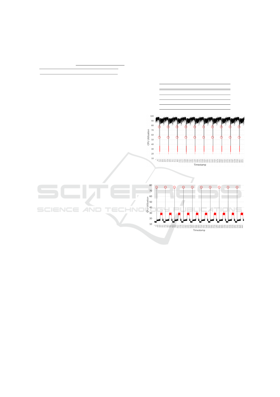
lies in B3B-10. Figures 3 and 4 illustrate the two time

series. Each point anomaly is marked as a red circle,

and each sequential anomaly is marked in red.

Table 1: Details of the two extended time series used in the

experiments.

Name CC2-10 B3B-10

# of data points 40320 40320

Time interval (min) 5 5

# of point anomalies 20 10

# of sequential anomalies 10 10

Figure 3: All data points of CC2-10. Note that all anomalies

are marked in red.

Figure 4: All data points of B3B-10. Note that all anomalies

are marked in red.

To achieve a fair comparison, all the three ap-

proaches had the same hyperparameter and param-

eter setting as listed in Table 2, and they were im-

plemented in DL4J (Deeplearning4j, 2023), which

is a programming library written in Java for deep

learning. All approaches adopted Early Stopping

(EarlyStopping, 2023) to automatically determine the

number of epochs (up to 50) for LSTM model train-

ing. Furthermore, the Look-Back parameter for both

RePAD and ReRe was set to three so that all the three

approaches always use three historical data points to

predict every upcoming data point. In both experi-

ments, RePAD2 was evaluated under four values for

variable W: 1440, 4032, 8064, and 16128. These slid-

ing window sizes are equivalent to 5, 14, 28, and 56

days because the number of data points collected per

day in both CC2 and B3B was 288. All the exper-

IoTBDS 2023 - 8th International Conference on Internet of Things, Big Data and Security

212

iments were performed on a laptop running MacOS

Monterey 12.6 with 2.6 GHz 6-Core Intel Core i7 and

16GB DDR4 SDRAM.

Table 2: The hyperparameter and parameter setting used by

the three approaches.

Hyperparameters and parameters Value

The number of hidden layers 1

The number of hidden units 10

The number of epochs 50

Learning rate 0.005

Activation function tanh

Random seed 140

To evaluate the detection accuracy of the three

approaches, we followed the evaluation method

used by (Lee et al., 2020a) to measure preci-

sion (which equals TP/(TP+FP)), recall (which

equals TP/(TP+FN)), and F-score (which equals

2×(precision×recall)/(precision+recall)). Note that

TP, FP, and FN represent true positive, false positive,

and false negative, respectively. More speciﬁcally, if

any point anomaly occurring at time point Z can be

detected within a time period ranging from time point

Z−K to time point Z+K, this anomaly is considered

correctly detected. On the other hand, for any sequen-

tial anomaly, if it starts at time point I and ends at time

point J (J>I), and it can be detected within a period

between I−K and J, this anomaly is considered cor-

rectly detected. Note that we followed (Ren et al.,

2019) and set K to 7. This setting was applied to all

the three approaches as well.

5.1 Experiment 1

Table 3 lists the detection accuracy of RePAD2,

RePAD, and ReRe on CC2-10. When W was 1440,

RePAD2 had a poor precision (i.e., 0.531). Even

though RePAD2 under this sliding window size had

recall of 1, the low precision resulted in the worst

F-score among all compared approaches. When W

was increased to 4032, the precision of RePAD2 sig-

niﬁcantly increased to 0.972, but its recall reduced

to 0.7, leading to the F-score of 0.814. We can see

that the detection accuracy of RePAD2 remained sim-

ilar when W was further increased to 8064, but it

dropped slightly when W was further increased to

16128. Based on the results shown in Table 3, we

can see that RePAD2 provides a slightly better de-

tection accuracy than RePAD when W is 4032, 8064,

or 16128. As compared with ReRe, RePAD2 offers

a comparable detection accuracy when W is 4032 or

8064.

To explain why RePAD2 has different results, Fig-

ures 5 − 8 illustrate how the detection threshold of

Table 3: The detection accuracy of different approaches on

CC2-10.

Approach Precision Recall F-score

RePAD2 (W=1440) 0.531 1 0.694

RePAD2 (W=4032) 0.972 0.7 0.814

RePAD2 (W=8064) 0.971 0.7 0.814

RePAD2 (W=16128) 0.965 0.7 0.811

RePAD 0.964 0.7 0.811

ReRe 0.971 0.7 0.814

RePAD2 changed over time under different values of

W. When W was 1440, we can see that the thresh-

old curve as shown in Figure 5 apparently rises and

then falls repeatedly, implying that RePAD2 period-

ically lost the memory about older historical AARE

values and obtained the memory about newer histor-

ical AARE values. Due to the fact that the detection

threshold was calculated at every time point based on

the past 1440 AARE values, the threshold was prone

to be affected by high AARE values. Such a phe-

nomenon caused a lot of false positives. That is why

RePAD2 with W of 1440 has poor precision.

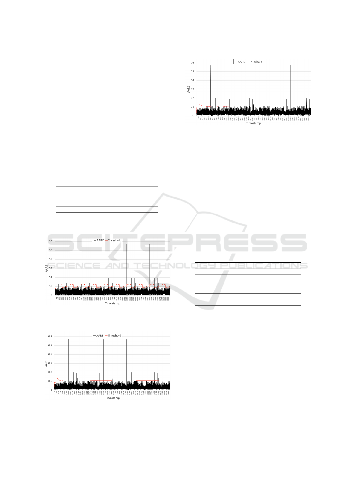
When W was increased to 4032 and 8064, the

threshold curve became ﬂatter (see Figures 6 and

7) since RePAD2 used more historical AARE val-

ues to calculate its detection threshold. In other

words, the threshold was less affected by few high

AARE values. However, when W was further in-

creased to 16128, it could not further improve the

precision of RePAD2 due to false positives. Never-

theless, RePAD2 achieves a similar detection accu-

racy as RePAD. Therefore, according to the results, it

is recommended to choose a sufﬁciently long sliding

window (e.g., 4032) for RePAD2 so as to reduce false

positives.

Figure 5: All derived AARE values vs. the detection thresh-

old over time when RePAD2 worked on CC2-10 and had a

sliding window of 1440.

Recall that RePAD2, RePAD, and ReRe are all de-

signed to decide if each upcoming data point in the

target time series is anomalous. When they ﬁnd that

their current LSTM models cannot accurately predict

a data point, they will retrain a new LSTM model.

Table 4 lists the LSTM retraining ratios of all the

RePAD2: Real-Time Lightweight Adaptive Anomaly Detection for Open-Ended Time Series

213

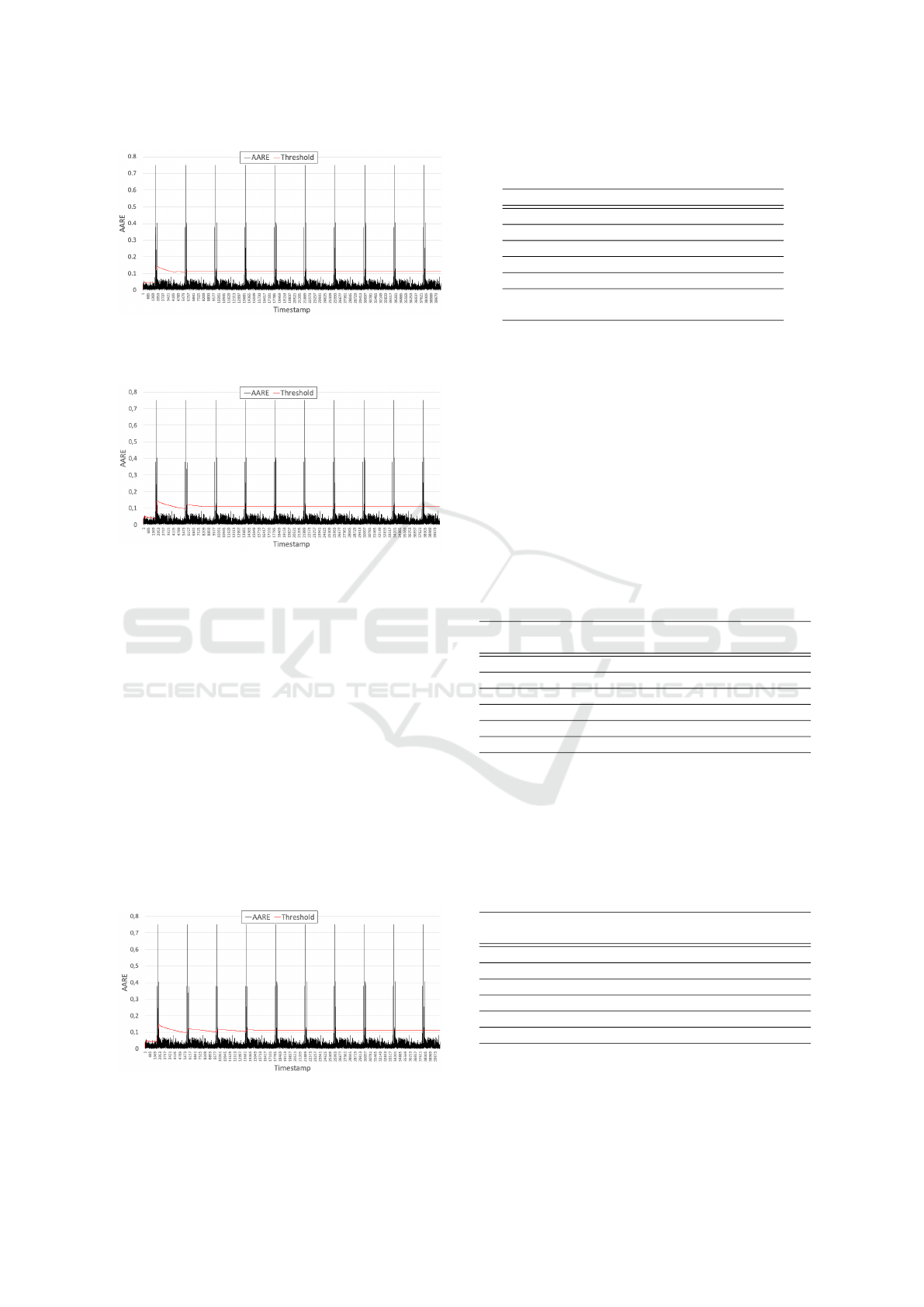
Figure 6: All derived AARE values vs. the detection thresh-

old over time when RePAD2 worked on CC2-10 and had a

sliding window of 4032.

Figure 7: All derived AARE values vs. the detection thresh-

old over time when RePAD2 worked on CC2-10 and had a

sliding window of 8064.

three approaches. When W was 1440, RePAD2 re-

quired to retrain a LSTM model for 555 data points.

Since the total number of the data points in CC2-10

is 40320, the LSTM model retraining ratio is 0.014.

We can see that the retraining ratio of RePAD2 re-

duced when W was increased, implying that including

more historical AARE values to calculate the thresh-

old helps reduce LSTM model retraining. When

RePAD2 is compared with RePAD, it requires slightly

more model retraining. But when it is compared with

ReRe, RePAD2 has a lower retraining ratio. This is

because ReRe employs two detectors to jointly detect

anomalies. The detection threshold used by detector

2 is more stricter than the detection threshold used by

detector 1, which causes more LSTM model retrain-

ing.

Figure 8: All derived AARE values vs. the detection thresh-

old over time when RePAD2 worked on CC2-10 and had a

sliding window of 16128.

Table 4: The LSTM training ratio of different approaches

on CC2-10.

Approach LSTM model retraining ratio

RePAD2 (W=1440) 0.014 (=555/40320)

RePAD2 (W=4032) 0.012 (=460/40320)

RePAD2 (W=8064) 0.011 (=448/40320)

RePAD2 (W=16128) 0.011 (=428/40320)

RePAD 0.010 (=417/40320)

ReRe 0.010 (=417/40320) for detector 1

0.038 (=1522/40320) for detector 2

Table 5 shows the average time required by the

three approaches to decide if a data point in CC2-

10 is anomalous when LSTM model retraining is re-

quired. We can see that the time required by RePAD2

slightly reduced when W was increased, implying that

including more AARE values to calculate the detec-

tion threshold slightly helps reduce the time consump-

tion of RePAD2. As compared with RePAD, RePAD2

is slightly more efﬁcient when W is 8064 or 16128.

On the other hand, ReRe consumed more time than

RePAD2 and RePAD since it employs two parallel de-

tectors (rather than one detector) to detect anomalies

simultaneously.

Table 5: Time consumption of different approaches on

CC2-10 when LSTM model retraining is required.

Approach Average time to decide if a

data point is anomalous (sec)

Standard de-

viation (sec)

RePAD2 (W=1440) 0.205 0.030

RePAD2 (W=4032) 0.204 0.031

RePAD2 (W=8064) 0.200 0.027

RePAD2 (W=16128) 0.200 0.026

RePAD 0.202 0.030

ReRe 0.231 0.394

Table 6 lists the time consumption of the three

approaches when LSTM model retraining is not re-

quired by these approaches. It is clear that RePAD2

has a similar performance as RePAD, but a slightly

better performance than ReRe.

Table 6: Time consumption of different approaches on

CC2-10 when LSTM model retraining is NOT required.

Approach Average time to decide if a

data point is anomalous (sec)

Standard de-

viation (sec)

RePAD2 (W=1440) 0.029 0.032

RePAD2 (W=4032) 0.028 0.012

RePAD2 (W=8064) 0.028 0.012

RePAD2 (W=16128) 0.028 0.011

RePAD 0.028 0.012

ReRe 0.031 0.080

Based on all the above results on CC2-10, we can

see that RePAD2 provides a slightly better detection

accuracy and/or a slightly less time consumption than

IoTBDS 2023 - 8th International Conference on Internet of Things, Big Data and Security

214

RePAD when it uses a sufﬁciently long sliding win-

dow (e.g., 4032, 8064, or 16128) to calculate its de-

tection threshold. As compared with ReRe, RePAD2

offers a comparable detection accuracy and a slightly

less time consumption when its sliding window size

is 4032 or 8064.

5.2 Experiment 2

In experiment 2, we evaluated the performance of the

three approaches on B3B-10. As listed in Table 7,

RePAD2 had poor precision when W was 1440. This

is because the threshold repeatedly rose and dropped

and when it dropped, its value was lower than 0.1 (see

Figure 9), which caused many false positives.

Table 7: The detection accuracy of different approaches on

B3B-10.

Approach Precision Recall F-score

RePAD2 (W=1440) 0.667 1 0.800

RePAD2 (W=4032) 0.920 1 0.958

RePAD2 (W=8064) 0.921 1 0.959

RePAD2 (W=16128) 0.939 1 0.969

RePAD 0.939 1 0.969

ReRe 0.939 1 0.969

Figure 9: All derived AARE values vs. the detection thresh-

old over time when RePAD2 worked on B3B-10 and had a

sliding window of 1440.

Figure 10: All derived AARE values vs. the detection

threshold over time when RePAD2 worked on B3B-10 and

had a sliding window of 4032.

When W was further increased to 4032 and 8064,

Figure 11: All derived AARE values vs. the detection

threshold over time when RePAD2 worked on B3B-10 and

had a sliding window of 8064.

the precision of RePAD2 signiﬁcantly increased to

0.920 and 0.921, respectively. We can see from Fig-

ures 10 and 11 that the two threshold curves are more

ﬂatter than that in Figure 9, and that the values of

the thresholds are higher than 0.1 in most of the time.

Hence, not so many normal data points were wrongly

identiﬁed as anomalous by RePAD2.

When W was further increased to 16128, RePAD2

achieved the same precision and recall (and of course

the same F-score) as RePAD and ReRe. Clearly, we

can see that increasing W helps increase the precision

of RePAD2.

Table 8: The LSTM training ratio of different approaches

on B3B-10.

Approach LSTM model retraining ratio

RePAD2 (W=1440) 0.006 (=225/40320)

RePAD2 (W=4032) 0.004 (=153/40320)

RePAD2 (W=8064) 0.004 (=152/40320)

RePAD2 (W=16128) 0.004 (=148/40320)

RePAD 0.004 (=148/40320)

ReRe 0.004 (=148/40320) for detector 1

0.008 (=323/40320) for detector 2

Table 8 shows the LSTM retraining ratios required

by the three approaches on B3B-10. Apparently,

RePAD2 required the most LSTM model retraining

when W was 1440, and we can also see from Ta-

ble 9 that these retraining slightly impacted the time

consumption of RePAD2. However, when W was in-

creased, the retraining ratio of RePAD2 reduced and

stabilized, and it is comparable to that of RePAD and

less than that of ReRe. In addition, we can also see

that the time consumption of RePAD2 (as shown in

Table 9) slightly reduced as W was increased, and

RePAD2 was slightly more efﬁcient than RePAD and

ReRe. Table 10 shows RePAD2 had almost the same

time consumption as RePAD when LSTM model re-

training was not required, regardless of the value of

Based on the above results on B3B-10, we con-

RePAD2: Real-Time Lightweight Adaptive Anomaly Detection for Open-Ended Time Series

215

Table 9: Time consumption of different approaches on

B3B-10 while LSTM model retraining is required.

Approach Average time to decide if a

data point is anomalous (sec)

Standard de-

viation (sec)

RePAD2 (W=1440) 0.207 0.023

RePAD2 (W=4032) 0.204 0.019

RePAD2 (W=8064) 0.203 0.023

RePAD2 (W=16128) 0.203 0.024

RePAD 0.206 0.026

ReRe 0.314 0.706

clude that RePAD2 can achieve the same detection

accuracy as RePAD and ReRe when it uses the slid-

ing window size of 16128, but it consumes less time

consumption than RePAD and ReRe, especially when

LSTM model retraining is required.

Table 10: Time consumption of different approaches on

B3B-10 while LSTM model retraining is NOT required.

Approach Average time to decide if a

data point is anomalous (sec)

Standard de-

viation (sec)

RePAD2 (W=1440) 0.028 0.010

RePAD2 (W=4032) 0.028 0.009

RePAD2 (W=8064) 0.028 0.009

RePAD2 (W=16128) 0.028 0.009

RePAD 0.028 0.010

ReRe 0.032 0.133

6 CONCLUSIONS AND FUTURE

WORK

In this paper, we have introduced RePAD2 for ad-

dressing the resource exhaustion problem that several

state-of-the-art real-time and lightweight anomaly de-

tection approaches might suffer when they work on

open-ended time series for a long time. By limiting

the number of historical AARE values to calculate the

detection threshold that is dynamically updated at ev-

ery data point (except for the ﬁrst few data points),

RePAD2 successfully avoids the underlying system

resources from exhaustion.

Two experiments based on real-world time series

from the Numenta Anomaly Benchmark have been

conducted to compare RePAD2 with two other real-

time and lightweight anomaly detection approaches

(i.e., RePAD and ReRe). Four different sliding win-

dow sizes were used to evaluate the performance of

RePAD2. According to the results, it is not recom-

mended that RePAD2 uses a small sliding window

size (i.e., using a few number of historical AARE val-

ues to calculate the detection threshold) because the

detection threshold will ﬂuctuate over time and it will

cause unwanted false positives.

A large sliding window size is recommended for

RePAD2. As compared with RePAD and ReRe,

RePAD2 with a large sliding window can reduce false

positives and increase F-score, and therefore offers ei-

ther slightly better or comparable detection accuracy.

In addition, RePAD2 provides a slightly better per-

formance when it comes to the time consumption for

determining whether each data point in the target time

series is anomalous or not.

As our future work, we would like to implement

and deploy RePAD2 on a tiny computer such as Rasp-

berry Pi for different IoT time series anomaly detec-

tion (e.g., energy consumption, network trafﬁc, room

temperature, humidity, etc.). We also plan to deploy

RePAD2 on android-based smart phones to see how

it can help individual user to better monitor their net-

work usages. In addition, we plan to extend RePAD2

to detect anomalies in multivariate open-ended time

series in a real-time and lightweight manner.

ACKNOWLEDGEMENTS

The authors want to thank the anonymous review-

ers for their reviews and valuable suggestions to this

paper. This work was supported by the S3UNIP

project - University Grant Package Smart Software

Systems funded by Høgskulen p

a Vestlandet (HVL)

under project number 5700036-19.

REFERENCES

Aggarwal, C. C. and Yu, P. S. (2008). Outlier detection

with uncertain data. In Proceedings of the 2008 SIAM

International Conference on Data Mining, pages 483–

493. SIAM.

Ahmed, M., Mahmood, A. N., and Hu, J. (2016). A survey

of network anomaly detection techniques. Journal of

Network and Computer Applications, 60:19–31.

Bontemps, L., Cao, V. L., McDermott, J., and Le-Khac,

N.-A. (2016). Collective anomaly detection based on

long short-term memory recurrent neural networks. In

International conference on future data and security

engineering, pages 141–152. Springer.

Deeplearning4j (2023). Introduction to core deeplearning4j

concepts. https://deeplearning4j.konduit.ai/. [Online;

accessed 24-February-2023].

EarlyStopping (2023). What is early stopping? https:

//deeplearning4j.konduit.ai/. [Online; accessed 24-

February-2023].

Fisher, W. D., Camp, T. K., and Krzhizhanovskaya, V. V.

(2016). Crack detection in earth dam and levee passive

seismic data using support vector machines. Procedia

Computer Science, 80:577–586.

IoTBDS 2023 - 8th International Conference on Internet of Things, Big Data and Security

216

Hawkins, D. M. (1980). Identiﬁcation of outliers, vol-

ume 11. Springer.

Hochenbaum, J., Vallis, O. S., and Kejariwal, A. (2017).

Automatic anomaly detection in the cloud via statisti-

cal learning. arXiv preprint arXiv:1704.07706.

Hochreiter, S. and Schmidhuber, J. (1997). Long short-term

memory. Neural computation, 9(8):1735–1780.

Laptev, N., Amizadeh, S., and Flint, I. (2015). Generic

and scalable framework for automated time-series

anomaly detection. In Proceedings of the 21th ACM

SIGKDD international conference on knowledge dis-

covery and data mining, pages 1939–1947.

Lavin, A. and Ahmad, S. (2015). Evaluating real-time

anomaly detection algorithms–the numenta anomaly

benchmark. In 2015 IEEE 14th international confer-

ence on machine learning and applications (ICMLA),

pages 38–44. IEEE.

Lee, M.-C., Lin, J.-C., and Gan, E. G. (2020a). ReRe: A

lightweight real-time ready-to-go anomaly detection

approach for time series. In 2020 IEEE 44th Annual

Computers, Software, and Applications Conference

(COMPSAC), pages 322–327. IEEE. arXiv preprint

arXiv:2004.02319. The updated version of the ReRe

algorithm from arXiv was used in this RePAD2 paper.

Lee, M.-C., Lin, J.-C., and Gran, E. G. (2020b). RePAD:

real-time proactive anomaly detection for time series.

In Advanced Information Networking and Applica-

tions: Proceedings of the 34th International Confer-

ence on Advanced Information Networking and Ap-

plications (AINA-2020), pages 1291–1302. Springer.

arXiv preprint arXiv:2001.08922. The updated ver-

sion of the RePAD algorithm from arXiv was used in

this RePAD2 paper.

Lee, M.-C., Lin, J.-C., and Gran, E. G. (2021a). How far

should we look back to achieve effective real-time

time-series anomaly detection? In Advanced Infor-

mation Networking and Applications: Proceedings of

the 35th International Conference on Advanced In-

formation Networking and Applications (AINA-2021),

Volume 1, pages 136–148. Springer. arXiv preprint

arXiv:2102.06560.

Lee, M.-C., Lin, J.-C., and Gran, E. G. (2021b). SALAD:

Self-adaptive lightweight anomaly detection for real-

time recurrent time series. In 2021 IEEE 45th An-

nual Computers, Software, and Applications Confer-

ence (COMPSAC), pages 344–349. IEEE.

Lee, T. J., Gottschlich, J., Tatbul, N., Metcalf, E., and

Zdonik, S. (2018). Greenhouse: A zero-positive ma-

chine learning system for time-series anomaly detec-

tion. arXiv preprint arXiv:1801.03168.

LinkedIn (2018). linkedin/luminol [online code reposi-

tory]. https://github.com/linkedin/luminol. [Online;

accessed 24-February-2023].

NAB (2015). numenta/nab [online code repository]. url=

{https://github.com/numenta/NAB}. [Online; ac-

cessed 24-February-2023].

Ren, H., Xu, B., Wang, Y., Yi, C., Huang, C., Kou, X., Xing,

T., Yang, M., Tong, J., and Zhang, Q. (2019). Time-

series anomaly detection service at microsoft. In Pro-

ceedings of the 25th ACM SIGKDD international con-

ference on knowledge discovery & data mining, pages

3009–3017.

Schneider, J., Wenig, P., and Papenbrock, T. (2021). Dis-

tributed detection of sequential anomalies in univari-

ate time series. The VLDB Journal, 30(4):579–602.

Siffer, A., Fouque, P.-A., Termier, A., and Largouet, C.

(2017). Anomaly detection in streams with ex-

treme value theory. In Proceedings of the 23rd

ACM SIGKDD International Conference on Knowl-

edge Discovery and Data Mining, pages 1067–1075.

Staudemeyer, R. C. (2015). Applying long short-term mem-

ory recurrent neural networks to intrusion detection.

South African Computer Journal, 56(1):136–154.

Twitter (2015). Twitter/anomalydetection [online

code repository]. https://github.com/twitter/

AnomalyDetection. [Online; accessed 24-February-

2023].

Wu, J., Zeng, W., and Yan, F. (2018). Hierarchical tem-

poral memory method for time-series-based anomaly

detection. Neurocomputing, 273:535–546.

Xu, J. and Shelton, C. R. (2010). Intrusion detection using

continuous time bayesian networks. Journal of Artiﬁ-

cial Intelligence Research, 39:745–774.

RePAD2: Real-Time Lightweight Adaptive Anomaly Detection for Open-Ended Time Series

217