Automatic Defect Detection in Sewer Network Using Deep Learning

Based Object Detector

Bach Ha

, Birgit Schalter

, Laura White

and Joachim K

ohler

NetMedia, Fraunhofer IAIS, Schloss Birlinghoven 1, 53757 Sankt Augustin, Germany

Dr.-Ing. Pecher und Partner Ingenieurgesellschaft mbH, Sachsendamm 93, 10829 Berlin, Germany

Keywords:

Object Detection, Automatic Defect Detection, Sewer Inspection, AI Based Process Optimization.

Abstract:

Maintaining sewer systems in large cities is important, but also time and effort consuming, because visual

inspections are currently done manually. To reduce the amount of aforementioned manual work, defects within

sewer pipes should be located and classiﬁed automatically. In the past, multiple works have attempted solving

this problem using classical image processing, machine learning, or a combination of those. However, each

provided solution only focus on detecting a limited set of defect/structure types, such as ﬁssure, root, and/or

connection. Furthermore, due to the use of hand-crafted features and small training datasets, generalization is

also problematic. In order to overcome these deﬁcits, a sizable dataset with 14.7 km of various sewer pipes

were annotated by sewer maintenance experts in the scope of this work. On top of that, an object detector

(EfﬁcientDet-D0) was trained for automatic defect detection. From the result of several expermients, peculiar

natures of defects in the context of object detection, which greatly effect annotation and training process, are

found and discussed. At the end, the ﬁnal detector was able to detect 83% of defects in the test set; out of the

missing 17%, only 0.77% are very severe defects. This work provides an example of applying deep learning-

based object detection into an important but quiet engineering ﬁeld. It also gives some practical pointers on

how to annotate peculiar ”object”, such as defects.

1 INTRODUCTION

Sewer systems in large cities require continuous enor-

mous amounts of maintenance; for example, in Berlin

650 km of sewer pipes must be inspected each year.

This inspection process is done by domain experts

viewing video recordings of pipe interiors and mark-

ing defects manually. Consequently, such a process is

time-consuming, tedious, and error-prone. In order to

reduce the amount of necessitated manual effort, mul-

tiple previous works attempted to automatically de-

fects using classical image processing methods, and

rudimentary machine learning on hand-crafted fea-

tures (Makar, 1999). As a result, each work is limited

to only one or two speciﬁc type of defects. General-

ization to changes in appearance of defects and back-

ground is also another potential issue. While classi-

cal image processing based works’ result are promis-

ing, they are not yet enough for practical use on the

ﬁeld. On the other hand, modern deep-learning based

works have also been developed as an attempt to solve

this task. While delivering good results, networks

from these works are trained and evaluated on rel-

atively small datasets (Cheng and Wang, 2018; Ku-

mar et al., 2020). Consequently, generalization, or

how networks behave to variation in inputs, is a po-

tential problem. In order to deal with the aforemen-

tioned deﬁcits, this work aimed to develop an auto-

matic deep learning (DL) based defect detector, which

is trained and evaluated on a new sizable and varied

dataset. This detector’s architecture is Efﬁcient-Det

D0 (Tan et al., 2020). Beside automatic evaluation,

the ﬁnal evaluation is also done by expert engineers

in the ﬁeld, thus providing a thorough and practical

report on the network’s performance. This paper is di-

vided into ﬁve main sections. Related work provides a

brief overview on the current status of automatic de-

fects detection in sewer systems, and deep learning

based vision object detection. The second section ex-

plains methodology, as well as accompanying prob-

lems for data acquisition, annotation, network train-

ing, and evaluation. Next are the result section, future

works section, and ﬁnally the conclusion.

188

Ha, B., Schalter, B., White, L. and Köhler, J.

Automatic Defect Detection in Sewer Network Using Deep Learning Based Object Detector.

DOI: 10.5220/0011986300003497

In Proceedings of the 3rd International Conference on Image Processing and Vision Engineering (IMPROVE 2023), pages 188-198

ISBN: 978-989-758-642-2; ISSN: 2795-4943

 2023 by SCITEPRESS – Science and Technology Publications, Lda. Under CC license (CC BY-NC-ND 4.0)

2 RELATED WORK

This section gives more details on previous works in

the ﬁeld of sewer maintenance that attempted to solve

the same problem and their deﬁcits. In addition, a

short overview on deep-learning based object detec-

tions is also provided.

2.1 Sewer Maintenance

In order to efﬁciently inspect inaccessible sewer

systems multiple non-destructive diagnostic methods

have been developed since at least 1981 (Makar,

1999). While systems making use of sensors, such as

ground penetrating radars, ultrasound, laser-scanner

(Duran et al., 2002; Bailey et al., 2011) have

been developed and applied, closed-circuit television

(CCTV) based methods (Makar, 1999) are more pop-

ular due to the intuitive nature of the data, which

can be manually analyzed by technicians. Earlier

CCTV based methods (Moselhi and Shehab-Eldeen,

1999; Sinha, 2000; Sinha et al., 1999; Yang and Su,

2008) made use of classical image processing such

as edge detection, or boundary segmentation to de-

tect the present of defects on pipes’ inner surface,

and perform feature extraction. After that, classiﬁca-

tion of defects are done either by using heuristic from

ﬁxed extracted features (size, diameters, etc.) (Sinha,

2000; M

uller and Fischer, 2009; Huynh et al., 2015;

Tung-Ching, 2015) or various machine learning tech-

nics, for example neural network (NN) (Moselhi and

Shehab-Eldeen, 1999; Hassan et al., 2019), fuzzy-

neural network (Sinha et al., 1999), radial basis net-

work (RBN), and support vector machine (SVM)

(Yang and Su, 2008; Hengmeechai, 2013). While

producing results, these classical/hybrid methods re-

quire careful choices and conﬁgurations of image pre-

processing methods based on deﬁned target types of

defects. In consequence, each resulting solution is

limited to one or two very speciﬁc types of defect (i.e.

ﬁssure, joint open, root). Furthermore, hand-crafted

conﬁgurations make the solution inﬂexible to varia-

tions in environments, and defects. Another problem

is that most of them depend on edge detection, which

make defects with similar forms, for example ﬁssure

and root, not differentiable. In recent years, such

shortcomings could potentially be solved using arti-

ﬁcial neural networks (ANN). Although neural net-

works were already mentioned and used, these net-

works are still working on top of hand-crafted fea-

ture vectors, thus continue to be limited by the orig-

inal conﬁguration. An explanation for such deci-

sions was the lack of computational power (Moselhi

and Shehab-Eldeen, 1999; Yang and Su, 2008) at the

time. A more recent paper (Hassan et al., 2019) has

been able to perform classiﬁcation directly on RGB

input images, however a technician is required to

control the camera view and locate potential defects.

Recently, thanks to advancements in hardware, con-

cerns over performance issues of neural networks are

less relevant. Which leads to the existence of mul-

tiple methods using complex deep neural networks

(DNN) (Kunzel et al., 2018; Cheng and Wang, 2018;

Kumar et al., 2020; Wang et al., 2021), which not

only classify but also localize defects simultaneously.

These newer methods feed camera images directly

into a FasterRCNN (Cheng and Wang, 2018; Kumar

et al., 2020; Wang et al., 2021), or YOLOv3 (Ku-

mar et al., 2020) object detection network, which pro-

duces bounding boxes representing location and clas-

siﬁcation of defects. However, these deep-learning

based methods used relatively small datasets, which

only focus on a small set of defects (ﬁssure, root, in-

ﬁltration, deposit), for training and evaluation. An-

other problem is that, these earlier network only pro-

vided a perspective view of part of detected defects or

complex defect system, which would not allow easy

automatic measurement and damage assessment. An-

other type of DNN that performs image segmentation,

namely FRRN (Kunzel et al., 2018), was also used in

an effort to detect sewer pipes’ defects. This method

however projects raw video images into a single 2D

unrolling of the pipe, similar to (M

uller and Fischer,

2009), which is then fed to the FRRN for segmenta-

tion. Regardless, the segmentation network from this

work has problem with overlapping defects.

2.2 DL Based Vision Object Detection

Detecting objects in RGB images produced by CCTV

is a suitable task for deep learning based object detec-

tors. These detectors are a subset of DNN, which spe-

cialize in localizing and classifying objects on visual

data, such as RGB images. There are currently three

main groups of such detectors, namely two-stage de-

tectors, one-stage detectors (Zhao et al., 2019), and

recently developed transformer-based detectors.

Two-stage detectors are networks such as FastR-

CNN (Girshick, 2015), or FasterRCNN (Ren et al.,

2015). These networks function somewhat similar to

classical image processing methods, by ﬁrst locating

region of interests (ROI), each of which is the location

of a potential object. Next, classiﬁcation is performed

on each ROI to get the object class. Thanks to the sep-

aration of localization and classiﬁcation functionality,

two-stage detectors can reliably provide accurate ob-

ject location and class. Two-stages networks’ training

process are also more stable and easier to control, be-

Automatic Defect Detection in Sewer Network Using Deep Learning Based Object Detector

189

cause the localization part and classiﬁcation part can

be trained separately. In return, they are slower and

require a more complicated training process.

On the other hand, one-stage detectors, such as

networks from the YOLO-family (Redmon et al.,

2016; Redmon and Farhadi, 2018), Single-Shot-

Detector (SSD) (Liu et al., 2016), or the EfﬁcientDet-

family (Tan et al., 2020), trade training stability for

better performance and a simpler training process by

performing both localization and classiﬁcation simul-

taneously. Being a uniﬁed calculation graph allowed

these networks to be optimized on lower software and

hardware level, thus greatly increasing their process-

ing speed. The same characteristic however makes

it difﬁcult to improve the localization and classiﬁca-

tion separately, since both parts have to be trained

together. Earlier one-stage detectors generally have

lower accuracy than two-stage detectors, however this

is no longer always true for newer iterations (Zhao

et al., 2019; Wang et al., 2022a).

The third and ﬁnal group, transformer detectors

are recently introduced networks, which makes use

of attention mechanism instead of pure convolutional

layers. One of the ﬁrst and most famous network

of this group is DETR (Carion et al., 2020). Since

then transformer-based detectors have consistently

produced highly accurate detections, and one of them

(Wang et al., 2022b) is currently at the top of the

COCO benchmark (Lin et al., 2014). However, these

networks are extremely large and much slower in

comparison to networks in the other two groups. Fur-

thermore, the required amount of data for training

them is also very high.

3 METHOD

Figure 1: New inspection workﬂow with automatic object

detector integration.

To satisfy the use-case, the to be designed solution has

to adhere to the following requirements. Firstly, the

system must allow technicians to pinpoint the location

of defects, as well as providing them with an overall

and clear view of defects. Secondly, produced detec-

tions should allow an accurate measurement of defect

size and length (i.e. of ﬁssures, and root). The third

requirement is that the annotation process for training

data should not be complicated and extremely time-

consuming. Next, the system should require minimal

controlling effort and time on site, avoiding closing

off the street for a long period of time. Finally, pro-

cessing of recorded video data should be efﬁcient and

done in a reasonable amount of time without the need

of expensive computation clusters.

With the aforementioned requirements in mind,

the following design choices were made. In order

to fulﬁll the ﬁrst and second requirements, the net-

work will not work directly on video frames, but

on unrolled 2D projections of pipes’ inner surface,

which was similarly done in (M

uller and Fischer,

2009; Kunzel et al., 2018). This method also re-

duces the amount of images, that have to be pro-

cessed by the neural network, because near identical

frames from camera recordings are eliminated. The

third and fourth requirements rule out the application

of segmentation neural networks in (Kunzel et al.,

2018). Because of the complexity and required ac-

curacy of segmentation masks, labeling at pixel level

is very time-consuming (Cordts et al., 2016) in com-

parison to drawing bounding boxes over defects. Seg-

mentation networks are also generally slower and re-

quire more computational resources in comparison to

bounding box (BB) based detectors. Therefore, BB-

based object detectors would be the more suitable

choice. The last two requirements directly exclude

transformer based networks, and favor single-stage

detectors over two-stages detectors; with the type of

detector narrowed down, there is still the choice of

the speciﬁc network architecture, such as SSD, Reti-

naNet (Lin et al., 2017), YOLO-Family, or Efﬁcient-

Det. EfﬁcientDet was chosen, because at the time

it was the current state-of-the-art (Tan et al., 2020).

However, it should be noted that newer versions of

YOLO (YOLOv5, YOLOv7 (Wang et al., 2022a)) are

also promising.

3.1 Dataset Acquisition and Annotation

Problems

For the purpose of training the chosen neural network,

a sewer defects detection dataset is constructed from

maintenance ﬁsheye videos of Berlin’s sewer system.

Before anything else is done, each video is unrolled

and stitched into a single W × 1200 RGB image using

the method described in (Kunzel et al., 2018). The

width W of each output image depends on the length

of each inspected pipe. With the RGB input for the

network secured, the next important step is obtain-

IMPROVE 2023 - 3rd International Conference on Image Processing and Vision Engineering

190

Figure 2: Visualization of data within the pipeline.

ing bounding box annotations. For this step, a set of

9 common defects and 1 structure element similar to

(Kunzel et al., 2018) is deﬁned. Defects include set-

tled deposits (BBC), break/collapse (BAC), deforma-

tion (BAA), obstacle (BBE), angular displaced joint

(BAJ C), surface damage (BAF), horizontal displaced

joint (BAJ B), ﬁssure (BAB), and root (BBA). While

structure element only consist of one class: connec-

tion (BCA). Name of all defects/structure are taken

from the English translation of the German standard:

”DIN EN 13508-2:2011-08” (DIN, 2011). While the

accompanied letter codes are from the Euronorm. In

total, the dataset includes 14.7 km of annotated sewer

pipes.

Figure 3: Distribution of defect types.

Beside the known large amount of effort needed to

annotate a machine learning dataset, the defects in this

dataset also introduce their own additional problems.

Although deﬁned as an object detection dataset, un-

like COCO(Lin et al., 2014) or KITTI(Geiger et al.,

2012) datasets, the task of drawing a box over an

object and assigning a class to it for this dataset is

not as straight forward, which cost a lot of time and

necessitated multiple iterations of annotations. The

main cause is the uncommon and sometime ambigu-

ous nature of defects within sewer pipes. Unlike nat-

ural objects such as cat, dog, or car, which mostly re-

quire only common sense, defects require training and

experience to be accurately diagnosed. This means

that the labeling process has to be carried out only

by maintenance experts to ensure higher annotations

quality. With that in mind, in order to accelerate the

labeling process, the ﬁrst iteration of annotation was

done by letting experts work in parallel on different

sewer pipes. That was a wrong decision that lead

to the failure of the ﬁrst iteration of annotation, in

which produced labels for defects are so inconsistent

that neural network become more confused after the

training. The ﬁrst problem is that, even to experts,

some defects are still ambiguous. In another word

some experts might classify an ”object” as a defect,

while others do not, which further conﬁrms the ﬁnd-

ing made in (M

uller et al., 2006). The second problem

is deciding on a way to draw bounding boxes con-

sistently, which sensibly represents relevant ”object”.

Speciﬁcally, this is a problem with annotating ﬁssure,

root, and surface damage. Thinking back to objects in

COCO or KITTI; although color, size, and orientation

of these objects are varied, they all have certain ﬁxed

shape, form, or ratio and can be separated into single

instances (for example, a cat, a dog, a bike, ...). On

the other hand, ﬁssure, root, and erosion exist mostly

in form of clusters, which can be of any shape, size,

and density. Therefore, it is not trivial to intuitively

deﬁne an ”instance” for these defects, which can then

be surrounded by a box. Without a consistent and uni-

ﬁed guideline, each expert labeled these clusters with

different levels of coarseness, further exacerbating the

level of inconsistency in the dataset. Therefore, it is

clear that common labeling rules must be set. From

analyzing existing labels, there are two possible di-

rections to annotate such defects. The ﬁrst direction

is to coarsely label each entire region of connected

defects within a single bounding box. The other di-

rection is to ﬁnely divide each cluster into multiple

smaller ”instances”, each of which is labeled by a

bounding box. Here, smaller instance is loosely de-

ﬁned as the largest continuous segments of defects,

which can be ﬁtted into a tight bounding box, that has

high ”defect to background” area ratio. Examples in

ﬁgure 4 help show the difference between these two

aforementioned labeling directions.

Although ﬁnely divided labels do seem excessive

in the example, this inconvenience is outweighed by

more precise detections. Preliminary training and

testing on a subset of the dataset shows that network

trained with coarse labels is unable to detect smaller

and ﬁner ﬁssures, roots, and erosion areas. In con-

trast, networks trained with ﬁnely divided clusters

are capable of detecting not only smaller defects but

Automatic Defect Detection in Sewer Network Using Deep Learning Based Object Detector

191

Figure 4: Examples for how ﬁssures could be labeled, either

coarsely (top) or ﬁnely (bottom).

also larger defect clusters. While detection of such

large clusters are represented with a lot of smaller

overlapping bounding boxes, that is still much bet-

ter than completely missing defects, especially when

these smaller boxes can later be combined using vari-

ous post-processing methods.

With all this hindsight, in order to deal with the

ambiguous factor of defects and variations in label-

ing style, a second round of annotations was done fol-

lowing a stricter labeling guideline, with all experts

working together as a single group and vote on every

annotated defect. As a result, the annotations from

the second round are empirically more consistent. Fi-

nally, with large problems of the dataset sorted out,

the next step is to train the neural network.

3.2 Neural Network Training

This subsection describes main steps and correspond-

ing conﬁguration to train the required detector. As

reasoned in the beginning of this section 3, a net-

work from the EfﬁcientDet family (Tan et al., 2020)

was trained to detect defects and structures within

sewer pipes, speciﬁcally EfﬁcientDet-D0 was used.

The training follows a standard procedure of multiple

steps.

Firstly, the whole dataset is split into a train set

and a test set. For large public datasets, splits are often

already chosen and provided (Lin et al., 2014; Geiger

et al., 2012). When that is not the case, splits are

generally generated randomly from the whole dataset.

For such a new and self labeled dataset, random split

was a decent choice, which costs little time and effort.

However, results of the ﬁrst few cross validations on

random test sets shown large and chaotic variations,

where the network achieves really high accuracy in

some rounds while completely failing to recognize se-

vere defects in others. After further inspecting those

automatic splits, it was found that due to difference in

rarity of each defect type and sewer pipe conditions,

characteristics of each random split changed drasti-

cally. For example, there are splits, where the major-

ity of break/collapse or obstacle are concentrated in

the test set, thus the network is tested on defects that

it was hardly trained on. On the other hand, the test

set could mostly consist of healthy pipes, in which

the network easily detected most of the scattered de-

fects. In both cases, these networks are all incompa-

rable, and the evaluation untrustworthy due to a lack

of stable baselines. Therefore, a set of ten representa-

tive sewer pipes were instead manually chosen and set

aside for evaluation. For clarity, representative means

that these pipes must contain all the relevant defects

and structure with good variation. Furthermore, pipes

with defect free sections are also included to make

sure that the resulting network does not wrongly mark

healthy pipe sections as damaged.

With data splits sorted out, the second step is pre-

processing, some light data augmentation, and feed-

ing the neural network with RGB images. This how-

ever cannot simply be done like with COCO or KITTI

because of the images’ length. Unrolled RGB images

of pipes have resolution of around 20000x1200 pixel

to 150000x1200 pixel, which are too large and sim-

ply result in Out-Of-Memory (OOM) error when fed

directly into a detection network. Therefore, the so-

lution is a simple sliding window approach with each

patch having the size of 1200x1200 pixel. There is

also a 50% overlap between each window, so that

each defect is likely to be in full view of the net-

work. After the original image is cut into multiple

patches, data augmentation is then applied to each

patch separately. Each input patch and their corre-

sponding annotation have a 25% chance to be ﬂipped

up-down and another separate 25% chance for left-

right ﬂipping. This minimal augmentation helps in-

crease the variety of the dataset without introducing

too much artiﬁcial artifacts, which might have un-

known adverse effects on new unknown data. One

ﬁnal step before the network gets to see the data is

down-sampling from 1200x1200 to 640x640. This

was done so that the detector can be trained with a

batch size larger than 1. Another added beneﬁt is that

the network also requires less time for inference and

training. While accuracy could suffer due to lowered

resolution, a preliminary test shown negligible change

after down-sampling.

The third step is conﬁguring the training with

IMPROVE 2023 - 3rd International Conference on Image Processing and Vision Engineering

192

plausible values of hyperparameters, that are suitable

for the dataset and available hardware. These hyper-

parameters can be roughly divided into two groups:

network hyperparams and trainer hyperparams. How-

ever, it should be noted, that both groups are not in-

dependent but greatly affect each other. To the ﬁrst

group, the network hyperparams are, for example,

weight initialization options, or batch normalization

(Ioffe and Szegedy, 2015) conﬁgurations. Within this

group, the most important hyperparam is weight ini-

tialization, which was set to use weights pre-trained

on COCO (Tan et al., 2020). While simpler meth-

ods, such as variations of random initialization exist,

they are better suited for new unknown architectures

(He et al., 2015). Since the chosen EfﬁcientDet-D0 is

already established, and it is already shown that trans-

fer learning greatly improves the ﬁnal trained network

(Tan and Le, 2019), pre-trained weights initializa-

tion is more logical. To be more speciﬁc, pre-trained

weights allow networks to reuse proven learned fea-

ture extractors. This spares the training from the ear-

lier divergence-prone phase, which also requires a

large amount of data. As a result, such initialization

is especially useful for small datasets, that do not nec-

essarily have enough samples to properly stabilize its

feature extractors from scratch. This is still the true

for the defect dataset in this work, despite the fact that

this dataset’s domain is entirely different from that

of normal datasets, namely COCO or KITTI (normal

scenes vs. sewer pipe’s inner surfaces). With the net-

work conﬁgured, trainer’s hyperparams are next. For

this group, training hardware, especially the graphical

processing unit (GPU), has a lot of says in the conﬁg-

uration. In this case, an Nvidia GTX Titan X GPU

with 12 GB of random access memory (RAM) was

used. Thanks to the previous down-sampling step,

a batch size of 3 is set for the training. The opti-

mizer is Adam (Kingma and Ba, 2014) with default

parameters as suggested in its original paper. While

there other optimizers like stochastic gradient descent

(SGD) (Ruder, 2016) and its variants exist, Adam is

shown to keep the training process stable with little to

no additional hyperparameter conﬁguration (Kingma

and Ba, 2014; Ruder, 2016), which is especially im-

portant when working with new unknown data.

The fourth and longest step in training a neural

network is waiting. The training process is super-

vised using a combination of loss log, mean average

precision (mAP) (Lin et al., 2014) calculation, ROC-

curve, sample outputs between epochs, and a cus-

tom practical metric (see section 3.3). This enables

early stopping of training, either manually or auto-

matically if performance reaches a plateau or wors-

ens. On the aforementioned GPU, with a total of

around 71300 training patches, each training took ap-

proximately seven days before being stopped.

The ﬁfth and ﬁnal step is evaluating the trained

network on the pre-deﬁned test set from section 3.1.

Evaluation provides a close estimation of trained net-

works’ quality, which enables informed decision on

whether the training is ﬁnished, or what has to be

done in the next training cycle to deal with network’s

deﬁcit. In object detection, the standard procedure for

this step is running newly trained networks on test set

to produce predictions. After that, the quality of these

predictions, and of the networks, are then determined

automatically using a quantiﬁed metric such as mAP.

While higher mAP generally means better network,

there are cases where the corresponding predictions

are not ideal despite high mAP (Redmon and Farhadi,

2018). Other metrics such as precision, recall, and

the harmonic f1 score also work well as indicators for

network’s quality. In addition to automatic mAP cal-

culation, manually examining predictions of a random

subset of the test set is often done to ensure the qual-

ity of trained networks. However, this standard proce-

dure is not directly applicable into this work, forcing

some changes, which make it more suitable for practi-

cal applications. The deﬁcit and corresponding solu-

tions for the evaluation procedure would be discussed

in the next subsection 3.3.

3.3 Problem with mAP and Network

Evaluation

Figure 5: Differences in experts’ annotations (top), and the

networks’ detections (bottom) of formless defects, in this

case surface damages, which are marked with pink boxes.

This section provides details on why the standard

evaluation is not suitable for this use case, and how

to it was dealt with. The ﬁrst sight of problem was

Automatic Defect Detection in Sewer Network Using Deep Learning Based Object Detector

193

detected by simply following the established proce-

dure, calculated mAP for all best trainings are around

only 5 mAP. Such low score normally indicates one or

more of the following problems, namely bad network

architecture, misconﬁguration of input images and la-

bels, and/or peculiar problems of the dataset. Bad

network architecture is unlikely the reason, since Ef-

ﬁcientDet is able to handle large and complex dataset

(Lin et al., 2014). Careful review of the preprocess-

ing pipeline conﬁrms no misconﬁguration of input

data. With other potential sources of problem ruled

out, the remaining and most likely the reason for low

mAP score is the dataset itself. Given all taken pre-

cautions during data gathering, as mentioned in sec-

tion 3.1, this raises the question of what exactly the

problem with the dataset would be. A step to answer-

ing this question is manually checking the network’s

detections and comparing those with the annotation.

This reveals a downside of using bounding boxes

(BB), and by extension BB-based mAP calculation,

for denoting formless and cluster-like defects (.i.e ﬁs-

sure, root, surface damage). Manual check conﬁrms

that the network is indeed able to detect those de-

fects and correctly denote defects areas with multiple

boxes, however these generated bounding boxes do

not have the exact conﬁguration of the ground truth

boxes on the same damaged areas. For example, net-

work draws a single large box while the annotation

has multiple smaller side by side boxes, or vice versa

(see ﬁgure 5). This is especially bad for long ﬁne ﬁs-

sures or roots that run diagonally across the surface.

Therefore, from a practical point of view, mAP does

not correctly represent the network’s quality, when

such formless defects are concerned. As a side note,

while mask annotation could have solved this prob-

lem, it does have other undesirable downsides, as

mentioned in the start of section 3. Another prob-

lem with mAP is that, it lacks an intuitive baseline

to compare against. The current highest achievable

mAP on the COCO dataset is 65.4 mAP (Wang et al.,

2022b), which only shows that, that new network is

better than EfﬁcientDet-D0 (at 34.6 mAP) at produc-

ing predictions closer to the ground truths. 34.6 mAP

does not mean that EfﬁcientDet-D0 can only correctly

detect 34.6 out of every 100 objects; that number is

evidently higher (Tan et al., 2020). The SoTA 65.4

mAP also does not necessarily mean a double in ac-

curacy in comparison to EfﬁcientDet-D0. Unlike, for

example, percentage where 50% means the network

handles half of given tasks correctly. All in all, mAP

has limited use in practical applications. Now that the

problem has been identiﬁed, the next part will go into

the solution.

With the SoTA metric deemed less suitable for

the job, it was decided that the ﬁnal round of eval-

uation must be done manually by maintenance ex-

perts. While time and effort costly, this eliminates

any uncertainty regarding a network’s quality. Iron-

ically, the smaller dataset size helps make this task

more manageable. However, it is not realistic to ex-

pect the experts to examine every single experimental

training with different hyperparameter conﬁgurations,

because that would be a lot of unnecessary work and

the waiting time for results would be too long. There-

fore, an automatic metric for internal quality estima-

tion during experimentation, which mAP was sup-

posed to be, need to be created. In practice, the ex-

act location, and amount of defects on pipes’ inner

surface is not required by the experts. For them, it

is enough, and more practical to know on which me-

ters of pipe defects exist, and of what type. Based on

suggestions from the experts, and publication (Berger

et al., 2020), it was determined that running kilome-

ters/ meters is a standard baseline for metrics in the

ﬁeld of sewer sanitation. Hence, for practical pur-

poses, the internal metric would be using running me-

ters as base. To calculate this metric, each pipe is

ﬁrst divided into multiple 600x1200 chunks. Each

chunk would then be evaluated separately and would

be marked as true positive (TP), false positive (FP),

true negative (TN), or false negative (FN) depend-

ing on bounding boxes predictions within the chunk.

A chunk is deemed as TP if it contains at least one

bounding box with the correct class of one of the de-

fects in that chunk; the exact location and total num-

ber of predictions would not be taken into considera-

tion. A FP is given when the network put bounding

boxes in a defect-free chunk. A chunk is marked as

TN when the network does not produce any bounding

boxes in a defect-free chunk. A TN is asserted when

the network failed to produce any bounding boxes in

a chunk with actual defect; this is also the worst case

that must be minimized. After all chunks are evalu-

ated, standard statistics, such as accuracy, precision,

or recall can be easily calculated.

Figure 6: An example of the running meter metric; TP:

Green, TN: Blue, FP: Yellow, and FN: Red.

While this metric is clearly too lax in comparison

to mAP for SoTA object detection, it is for experts in

ﬁeld of sewer system more understandable and use-

ful. Intuitively, what this metric says is, that within all

pipe sections of N meters, X% of them have defects,

which are most likely of the following Y, Z type. With

IMPROVE 2023 - 3rd International Conference on Image Processing and Vision Engineering

194

Table 1: Expert’s evaluation on test set; precision and recall

for each defect/structural class. Statistics calculated from

evaluation results provided by the Dr.-Ing. Pecher und Part-

ner Ingenieurgesellschaft mbH.

Defects/Struct. Precision Recall N object

Fissure 0.6697 0.6854 154

Root 0.7182 0.8778 129

Connection 0.9565 1. 51

Ang. dis. joint 1. 0.04 25

Break/collapse 0.037 0.5 2

Deformation 0. 0. 3

Hor. dis. joint 0.5659 0.9626 4

Settled deposit 0. 0. 43

Surface damage 0.8903 0.8406 80

Obstacle 0.6875 0.7952 78

All average 0.5525 0.5702 569

that knowledge, experts could then directly go to the

marked section to perform thorough inspection, thus

making the ﬁnal decision on whether that pipe section

is to be ﬁxed or not.

To sum up, in this work, each trained network

would ﬁrst be automatically evaluated using the run-

ning meters metric. The promising ones are then sent

to experts for the ﬁnal and real evaluation. With the

method and metrics for evaluation deﬁned, the next

section would describe the ﬁnal defect detection re-

sult.

4 RESULT

This section report archived performance of the ﬁ-

nal network in terms of the running meters metric

and manual evaluation from the sewer inspection ex-

perts. Furthermore, analysis of the result and com-

ment on characteristics of different types of defect are

also given. While comparison with results from rele-

vance existing methods (Cheng and Wang, 2018; Ku-

mar et al., 2020; Wang et al., 2021) would be useful

and informative, this could not be done cleanly due

to a the lack of a common train/test dataset, as men-

tioned in subsection 2.1. To deal with this potential

deﬁcit, it is important to stress, that this paper leans

into the current most reliable and trusted evaluators:

domain experts. On the whole, the evaluation com-

prises 10 sewer pipes with a total number of 1549 de-

fects/structures detected by the experts. According to

the running meters metric, for a total of 1147 pipe sec-

tions, the network is able to produce 391 TP (34%),

447 TN (39%), 126 FP (11%), and 188 FN (16%). In

total, the accuracy is at 73.06%.

A numerical summary of the expert’s ﬁnal evalu-

ation can be seen in table 1. According to the experts,

Table 2: Severeness of the network’s false negatives. Table

provided by the Dr.-Ing. Pecher und Partner Ingenieurge-

sellschaft mbH.

Object count Condition class Severity

1 0 very severe

11 1 severe

159 2 & 3 med. & slight

90 4 minor

the total count of the network’s detections is consid-

erably higher than the manual detections by the ex-

perts: frequently, network produces multiple overlap-

ping detections for a single defect, or in other cases

a single defect is covered by several non-overlapping

detections. As a rule, network’s detections with very

low conﬁdence score (<= 10%) are negligible false

positives, and therefore are not part of the expert’s

evaluation. Out of the 1549 defects/structures from

the experts, 261 (17%) were not found by the network

and therefore are classiﬁed as false negatives. In table

2, the severity of these false negatives is classiﬁed ac-

cording to (DWA, 2007). Most of the false negatives

are classiﬁed as condition class 2 to 4, medium to

minor defects with no immediate or short-term need

of sanitation/renovation action; counting only severe

false negatives the number drops to 12 out of 1549

(0.77%). This concludes the summarized evaluation

result from the experts.

This paragraph goes into analyzing the result on

each type of defects/structure separately. Possible

performance affecting factors, and respective poten-

tial remedies are also presented. First, defect types

can be sorted into different categories. Except for

connection, which is a structural part of the pipe, the

nine defects class can be divided into 2 subgroups,

which partially explains the difference in network’s

reaction to each class. These subgroups are ﬂat (2D)

defects, and spatial (3D) defects. The difference be-

tween the two groups is, that spatial defects’ one

prominent feature is the offset between their surface

and the normal pipe surface; for example, how high

a pile of settled deposits is in the pipe, or how much

material is gone from the inner surface of the pipe.

However, this third dimension is lost during the un-

rolling processing. The ﬂat defects group includes

ﬁssure, root. On the other hand, spatial defects in-

cludes: angular displaced joint, settled deposit, sur-

face damage, break/collapse, deformation, horizontal

displaced joint, and obstacle In the ﬂat defects group,

the network is able to handle root quite well. The

performance on ﬁssure, however, still has room for

improvement, speciﬁcally on ﬁner and smaller ﬁs-

sures. Within spatial defects, the network is able to

detect surface damages, and obstacle quite well, de-

Automatic Defect Detection in Sewer Network Using Deep Learning Based Object Detector

195

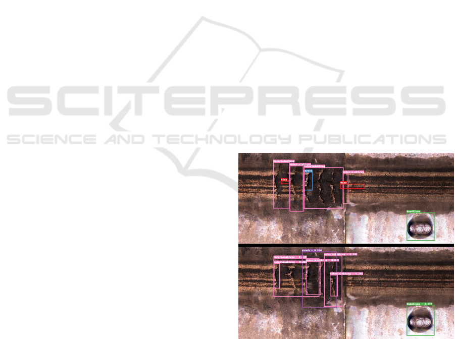
Figure 7: Visualization of experts’ annotations (left) and the networks’ detection (right) on a pipe section with multiple

defects.

spite the loss of spatial information. Surface damages

are generally easy for the network to detect due to

differences of coloration and texture in comparison

to healthy pipe surface. Obstacles are also detected

quite well, although it is a diverse class with multiple

subclasses of very different visual characteristics, for

example, encrustation, root balls, protruding shards

and crossing pipes. The ﬁrst reason is that, accord-

ing to the experts, they are easier to be detected in

2D images, thus less affected by the loss of spatial

information. Another possible explanation is that ob-

stacles usually appear with other defects, .i.e root and

root balls, thus detection of obstacles could be gener-

ated based on the existence of other relevant well de-

tected classes. The amount of available training sam-

ples for both surface damage, and obstacles could also

have positively contributed to the result. On the other

hand, most of the spatial defects are detected poorly

by the network. The most likely cause of this is the

mentioned loss of depth information. Furthermore,

these defects are also much rarer, thus having fewer

training samples. However, according to the experts,

deformations and horizontal displaced joints should

still be detectable without spatial data. Thus, the more

likely reason for bad performance is the lack of train-

ing data. The settled deposit class is especially bad,

despite having a somewhat sufﬁcient amount of train-

ing samples, the network failed to ﬁnd any of those

at all. Break/collapses are also in a bad position; the

network often mistakes chipped connection branches

or chipped joints in stone pipe for this type of de-

fects. Outside of defects, the single structural class,

connection, is handled easily by the network. Due

to their standardized features, connections are consis-

tence, unambiguous, and easy to label. In all relevant

classes, connection is the closest to a typical object

class in COCO or KITTI. As a side note, the ﬁnal

net’s mAP@0.5, mAP@0.75, and mAP@[.5 : .95] are

12.6, 5.5, and 5.8 respectively.

5 FUTURE WORK

This section presents some possible ways forward,

including general neural network improvements and

suggested heuristics from the sewer maintenance ex-

perts. These potential improvements can be coarsely

applied to one of the following areas: the neural net-

work and the post-processing. For the network itself,

accuracy could be raised by adding more high quality

annotated data, especially for rarer defects. On top of

that, several defect classes could be divided into more

speciﬁc subclass for better differentiation; for exam-

ple roots can be broken down to tap roots, indepen-

dent ﬁne roots, or complex mass of roots. While gen-

erally sensible, this method necessitates the need for

a lot more training data, and rework of current anno-

tated dataset. The third boost of accuracy could come

from preventing the loss of spatial information during

the unrolling; one way of achieving this would be us-

ing an RGBD camera or a stereo camera instead of

a normal RGB camera. This would greatly improve

the performance on spatial defects. Furthermore, ac-

cording the experts, adding the 3rd dimension would

also signiﬁcantly improve performance of ﬂat defects,

such as ﬁssures. Another chance of improvement can

also be from trying out newer SoTA network like

YOLOv5, or YOLOv7 (Wang et al., 2022a), etc.;

nonetheless, given the same dataset, there would be

no guarantee of a large jump in detection quality.

During evaluation, the experts also noticed several

undesirable behaviors from the network, which when

IMPROVE 2023 - 3rd International Conference on Image Processing and Vision Engineering

196

rectiﬁed would greatly improve the performance and

ease-of-use. In any case, these are concrete rules and

heuristics that could not be easily integrated directly

into the training, because the NN training process fo-

cuses on making networks learn abstract rules from

training data implicitly. As a result, the easiest way

for these explicit heuristics to be implemented would

be as post-processing steps after the detection. Ac-

cording to the experts, ﬁssures and surface damages

are often detected in small parts and/or multiple times.

This situation could possibly be corrected using clas-

sical methods such as Hungarian algorithm or con-

nected components to automatically merge relevant

detections together. Another suggestion is ﬁnding a

way to optimally set the minimum conﬁdence thresh-

old, which stems from the need to avoid overloading

the experts with too many false positives. Since each

type defect are handled differently, it would also be

useful to ﬁgure out one threshold for each defect type.

An additional problem with the network is, that de-

fects on the ceiling of pipes are divided into two parts.

This is caused by trying to project a continuous cylin-

der into 2D space; while circular image convolution

would be an interesting research topic, an easier way

of ﬁxing this could be using Hungarian algorithm, or

similar matching algorithms to match detections on

pipe’s ceiling. Finally, the following list contains sev-

eral practical heuristic rules directly from the experts,

which could be implemented to further better the ﬁnal

detection:

• Roots can only be detected in the immediate joint

and branch connection area.

• Circumferential ﬁssures are not observed in the

immediate vicinity of joints, as joints pick up

forces that lead to circumferential ﬁssures at other

parts of the sewer pipe.

• In the joint area of vitriﬁed clay pipe, ﬁssures

could form due to shrinkage of the glaze while

the pipe is cooling down after the ﬁring process.

These ﬁssures are only on the glaze, thus are un-

problematic to pipes’ structural stability.

• There is a strong correlation between material of

pipes, as well as locations within pipes and types

of defect that would appear. For example, con-

crete pipes are susceptible to chemical corrosion,

thus showing more surface damages over time.

On the other hand, while resistant to chemical

corrosion, vitriﬁed clay pipes are brittle. Conse-

quently, most defects found in these pipes are me-

chanical wear and tear, such as ﬁssures.

All in all, however complex and precise, post-

processing still has to rely on a good detection base-

line, as an extension the network.

6 CONCLUSIONS

In this work, an EfﬁcientDet-D0 was used to detect

defects on sewer pipes’ inner surface. This network

was trained on a new dataset of 14.7 km of sewer

pipe, which was manually annotated by expert in the

ﬁeld. At the end, the network is able to produce good

detections of ﬁssure, root, surface damage, obstacle,

and connection. However, other relevant defects with

spatial feature are still difﬁcult, due to the lack of

depth information. This problem could potentially

be solved using RGB-D camera. Furthermore, mul-

tiple post-processing using known practical heuris-

tics could also be applied to further improve detection

quality. Finally, this work also provided some prac-

tical designs for processing and evaluating ”objects”

with peculiar nature, such as defects.

ACKNOWLEDGEMENTS

This work is funded by the German Federal Min-

istry of Education and Research under grant number

13N13891.

REFERENCES

Bailey, D., Jones, M., and Tang, L. (2011). Real time vi-

sion for measuring pipe erosion. In The 5th Interna-

tional Conference on Automation, Robotics and Ap-

plications, pages 486–491. IEEE.

Berger, C., Falk, C., Hetzel, F., Pinnekamp, J., Ruppelt,

J., Schleiffer, P., and Schmitt, J. (2020). Zustand

der kanalisation in deutschland - ergebnisse der dwa-

umfrage 2020. Deutsche Vereinigung f

ur Wasser-

wirtschaft, Abwasser und Abfall e. V., 67:939–953.

Carion, N., Massa, F., Synnaeve, G., Usunier, N., Kirillov,

A., and Zagoruyko, S. (2020). End-to-end object de-

tection with transformers. CoRR, abs/2005.12872.

Cheng, J. C. and Wang, M. (2018). Automated detection

of sewer pipe defects in closed-circuit television im-

ages using deep learning techniques. Automation in

Construction, 95:155–171.

Cordts, M., Omran, M., Ramos, S., Rehfeld, T., Enzweiler,

M., Benenson, R., Franke, U., Roth, S., and Schiele,

B. (2016). The cityscapes dataset for semantic urban

scene understanding. CoRR, abs/1604.01685.

DIN (2011). Investigation and assessment of drain and

sewer systems outside buildings - part 2: Visual in-

spection coding system; EN 13508-2:2003+A1:2011.

Duran, O., Althoefer, K., and Seneviratne, L. (2002). Auto-

mated sewer pipe inspection through image process-

ing. volume 3, pages 2551–2556 vol.3.

DWA (2007). DWA-M 149-3E: Conditions and assessment

of drain and sewer systems outside buildings–part 3:

Condition classiﬁcation and assessment.

Automatic Defect Detection in Sewer Network Using Deep Learning Based Object Detector

197

Geiger, A., Lenz, P., and Urtasun, R. (2012). Are we ready

for autonomous driving? the kitti vision benchmark

suite. In 2012 IEEE Conference on Computer Vision

and Pattern Recognition, pages 3354–3361.

Girshick, R. B. (2015). Fast R-CNN. CoRR,

abs/1504.08083.

Hassan, S. I., Dang, L. M., Mehmood, I., Im, S., Choi, C.,

Kang, J., Park, Y.-S., and Moon, H. (2019). Under-

ground sewer pipe condition assessment based on con-

volutional neural networks. Automation in Construc-

tion, 106:102849.

He, K., Zhang, X., Ren, S., and Sun, J. (2015). Delving deep

into rectiﬁers: Surpassing human-level performance

on imagenet classiﬁcation. CoRR, abs/1502.01852.

Hengmeechai, J. (2013). Automated Analysis of Sewer In-

spection Closed Circuit Television Videos Using Im-

age Processing Techniques. PhD thesis, Faculty of

Graduate Studies and Research, University of Regina.

Huynh, P., Ross, R., Martchenko, A., and Devlin, J. (2015).

Anomaly inspection in sewer pipes using stereo vi-

sion. In 2015 IEEE International Conference on

Signal and Image Processing Applications (ICSIPA),

pages 60–64. IEEE.

Ioffe, S. and Szegedy, C. (2015). Batch normalization: Ac-

celerating deep network training by reducing internal

covariate shift. CoRR, abs/1502.03167.

Kingma, D. P. and Ba, J. (2014). Adam: A method for

stochastic optimization. arXiv:1412.6980.

Kumar, S. S., Wang, M., Abraham, D. M., Jahanshahi,

M. R., Iseley, T., and Cheng, J. C. (2020). Deep

learning–based automated detection of sewer defects

in cctv videos. Journal of Computing in Civil Engi-

neering, 34(1):04019047.

Kunzel, J., Werner, T., Eisert, P., and Waschnewski, J.

(2018). Automatic analysis of sewer pipes based on

unrolled monocular ﬁsheye images. In 2018 IEEE

Winter Conference on Applications of Computer Vi-

sion (WACV), pages 2019–2027. IEEE.

Lin, T., Goyal, P., Girshick, R. B., He, K., and Doll

ar, P.

(2017). Focal loss for dense object detection. CoRR,

abs/1708.02002.

Lin, T., Maire, M., Belongie, S. J., Bourdev, L. D., Girshick,

R. B., Hays, J., Perona, P., Ramanan, D., Doll

ar, P.,

and Zitnick, C. L. (2014). Microsoft COCO: common

objects in context. CoRR, abs/1405.0312.

Liu, W., Anguelov, D., Erhan, D., Szegedy, C., Reed, S.,

Fu, C.-Y., and Berg, A. C. (2016). SSD: Single Shot

MultiBox Detector. arvix, 9905:21–37.

Makar, J. M. (1999). Diagnostic techniques for sewer sys-

tems. Journal of Infrastructure Systems, 5:69–78.

Moselhi, O. and Shehab-Eldeen, T. (1999). Automated de-

tection of surface defects in water and sewer pipes.

Automation in Construction, 8(5):581–588.

uller, K. and Fischer, B. (2009). Objective condition as-

sessment of sewer systems. Strategic Asset Manage-

ment of Water Supply and Wastewater Infrastructures.

uller, K., Fischer, B., Lehmann, T., Hunger, W., and

Sch

afer, T. (2006). Forschungsprojekt bilderkennung-

ergebnisse der ersten projektphase. B I UmweltBau,

Redmon, J., Divvala, S., Girshick, R., and Farhadi, A.

(2016). You Only Look Once: Uniﬁed, Real-Time

Object Detection. arvix. arXiv:1506.02640 [cs] ver-

sion: 5.

Redmon, J. and Farhadi, A. (2018). YOLOv3: An Incre-

mental Improvement. arvix. arXiv:1804.02767 [cs].

Ren, S., He, K., Girshick, R. B., and Sun, J. (2015). Faster

R-CNN: towards real-time object detection with re-

gion proposal networks. CoRR, abs/1506.01497.

Ruder, S. (2016). An overview of gradient descent opti-

mization algorithms. CoRR, abs/1609.04747.

Sinha, S., Karray, F., and Fieguth, P. (1999). Under-

ground pipe cracks classiﬁcation using image anal-

ysis and neuro-fuzzy algorithm. In Proceedings of

the 1999 IEEE International Symposium on Intelli-

gent Control Intelligent Systems and Semiotics (Cat.

No.99CH37014), pages 399–404.

Sinha, S. K. (2000). Automated underground pipe inspec-

tion using a uniﬁed image processing and artiﬁcial in-

telligence methodology. University of Waterloo.

Tan, M. and Le, Q. V. (2019). Efﬁcientnet: Rethink-

ing model scaling for convolutional neural networks.

CoRR, abs/1905.11946.

Tan, M., Pang, R., and Le, Q. V. (2020). Efﬁ-

cientDet: Scalable and Efﬁcient Object Detection.

arXiv:1911.09070 [cs, eess] version: 7.

Tung-Ching, S. (2015). Segmentation of crack and open

joint in sewer pipelines based on cctv inspection im-

ages. In 2015 AASRI International Conference on

Circuits and Systems (CAS 2015), pages 263–266. At-

lantis Press.

Wang, C.-Y., Bochkovskiy, A., and Liao, H.-Y. M. (2022a).

Yolov7: Trainable bag-of-freebies sets new state-of-

the-art for real-time object detectors.

Wang, M., Luo, H., and Cheng, J. C. (2021). Towards an

automated condition assessment framework of under-

ground sewer pipes based on closed-circuit television

(cctv) images. Tunnelling and Underground Space

Technology, 110:103840.

Wang, W., Dai, J., Chen, Z., Huang, Z., Li, Z., Zhu, X.,

Hu, X., Lu, T., Lu, L., Li, H., et al. (2022b). In-

ternimage: Exploring large-scale vision foundation

models with deformable convolutions. arXiv preprint

arXiv:2211.05778.

Yang, M.-D. and Su, T.-C. (2008). Automated diagnosis

of sewer pipe defects based on machine learning ap-

proaches. Expert Systems with Applications.

Zhao, Z.-Q., Zheng, P., Xu, S.-T., and Wu, X. (2019). Ob-

ject detection with deep learning: A review. IEEE

Transactions on Neural Networks and Learning Sys-

tems, 30(11):3212–3232.

IMPROVE 2023 - 3rd International Conference on Image Processing and Vision Engineering

198