Impacts of Connected Automated Vehicles on Large Urban Road

Network

Qiong Lu

, Alessio Tesone

and Luigi Pariota

Department of Civil and Environmental Engineering, University of Naples Federico II, Naples, Italy

Keywords:

CAV, Large Urban Network, Maximum ﬂow, Average Speed, Congestion Duration, Over-Saturation Degree.

Abstract:

As an essential component of the Cooperative Intelligent Transportation System (C-ITS), Connected Auto-

mated Vehicles (CAVs) are anticipated to play a signiﬁcant role in the development of the future mobility

service. This paper investigates the impacts of different penetration of CAVs on the urban road network. The

investigation is carried out in a vast urban network with Simulation of Urban MObility (SUMO), a microscopic

trafﬁc simulator. The estimated factors of the network are network maximum ﬂow, critical density, average

speed, congestion duration, and roadway over-saturation degree. The Macroscopic Fundamental Diagram

(MFD) has been used to estimate the maximum ﬂow and critical density. In a simulation way, it substantiated

that a road network could have less scattered MFDs, even if the trafﬁc ﬂow is distributed heterogeneously. The

congestion duration and over-saturation degree are used to check trafﬁc congestion. The simulation results

show that applying 100% CAVs can contribute about a 13.55% increase in maximum ﬂow. A similar trend

can be found in the critical density for different CAV penetration rates. In a similar congestion situation, the

network with 100% CAV driving in can carry more than 130% of the original travel demand. In terms of

congestion level, even a low CAV penetration rate may signiﬁcantly improve the trafﬁc condition.

1 INTRODUCTION

Nowadays, researchers support Connected Auto-

mated Vehicles (CAVs) improvements in trafﬁc safety

and efﬁciency. However, quantifying the impacts of

CAVs is highly challenging. The challenge comes

from the uncertainty of how automated vehicles will

be introduced into our lives. For example, how will

the CAVs drive actually? Moreover, how will the

current trafﬁc management methods change with the

CAVs, how will the road authorities minimize the

infrastructure required for the mixed trafﬁc of man-

ual vehicles and automated vehicles, and the uncer-

tainty of CAV behaviors from different CAV com-

panies, etc.? Thus, the impacts of CAVs on trafﬁc

should be ﬁrst studied extensively. In the absence of

precise and massive amounts of data, a common way

to achieve this aim in current research is to perform

studies based on microscopic trafﬁc simulation tools

(Raju and Farah, 2021).

CAV microscopic simulation studies were con-

ducted on many trafﬁc topics, including ramp me-

https://orcid.org/0000-0002-0736-4320

https://orcid.org/0000-0002-8093-8175

https://orcid.org/0000-0001-9173-666X

tering(Liu et al., 2018; Xie et al., 2017), car fol-

lowing (Milan

es and Shladover, 2014; Wang et al.,

2015), trafﬁc signals (Goodall et al., 2013), emissions

(Mersky and Samaras, 2016), road safety (Papadoulis

et al., 2019), and mixed trafﬁc (Ye and Yamamoto,

2018). Most studies have differentiated CAVs and

human-driven vehicles (HDVs) by assuming that the

CAV driving behavior is less stochastic and consis-

tent. Simultaneously, CAVs have good lane disci-

pline.

Researchers used two main ways to model CAVs:

modifying the traditional car following and lane

changing models by adapting their parameters to the

supposed CAVs behavior (Lu et al., 2020), or by

deﬁning some novel models directly to mimic CAVs

behavior (Treiber et al., 2000; Van Arem et al., 2006).

Some researchers modeled CAVs by changing the pa-

rameters of the inbuilt car-following models. How-

ever, the simulated CAVs were less realistic in com-

parison to the ﬁeld behavior. The other researchers

applied numerous external algorithms to model the

CAVs. The main aim of the algorithms was to induce

communication among the vehicles. The CAVs were

governed by various models, including the Intelligent

Driver Model (IDM) (Treiber and Kesting, 2013),

378

Lu, Q., Tesone, A. and Pariota, L.

Impacts of Connected Automated Vehicles on Large Urban Road Network.

DOI: 10.5220/0011988000003479

In Proceedings of the 9th International Conference on Vehicle Technology and Intelligent Transport Systems (VEHITS 2023), pages 378-385

ISBN: 978-989-758-652-1; ISSN: 2184-495X

 2023 by SCITEPRESS – Science and Technology Publications, Lda. Under CC license (CC BY-NC-ND 4.0)

the Optimum Velocity Model (OVM) (Maske et al.,

2019), Adaptive Cruise Control (ACC) (Van Arem

et al., 2006), Cooperative Adaptive Cruise Control

CACC.

Of course, the presence of CAVs, once seen ag-

gregately, alters the performance of supply elements,

such as link cost functions and network performances.

The impacts of CAVs have been investigated recently.

For instance, several researchers have investigated the

CAV’s impacts on the freeway capacity (Ghiasi et al.,

2017; Chen et al., 2017). Shi and Li (2021) pro-

posed a method to construct a freeway Fundamen-

tal Diagram for trafﬁc ﬂow mixed with AVs. They

analyzed 3 data sets related to different time head-

way values for CAVs. They concluded that differ-

ent headway settings would mainly affect road ca-

pacity. Hu et al. (2021) analyzed the changes in the

Macroscopic Fundamental Diagram (MFD) of an ur-

ban corridor with the HDVs and CAVs mixed trafﬁc

ﬂow. The majority of the simulation results demon-

strate that the road capacity has been improved with

the growth of the CAVs penetration rate, the increase

of CAVs platoon intensity, and the reduction of head-

way time. However, the conclusions are also different

due to the different settings of the time headway for

CAVs. Lu et al. (2020) had investigated the impacts of

AVs on the MFDs of urban road networks. The paper

assumed that AVs have a shorter time headway and

concluded that AVs’ popularization would enlarge the

network capacity. Mavromatis et al. (2020) investi-

gated the impact of AVs and CAVs on ﬁve large urban

networks (about 3 km × 3 km). They found CAVs

can signiﬁcantly enlarge the trafﬁc ﬂow, decrease the

average trip time and reduce congestion. However,

they have yet to investigate the change in travel de-

mand that the road network can afford with the ap-

plication of CAVs. Tympakianaki et al. (2022) pro-

posed a framework to estimate the impacts of CAVs

on urban network performance. They investigated the

effects of the different penetration rates of CAVs on

network capacities. They found positive effects on ca-

pacities with the deployment of CAVs. Nevertheless,

the demand durations of the research on the impacts

of CAVs on large urban networks were only 1 hour

(Mavromatis et al., 2020; Tympakianaki et al., 2022).

There is a lack of research on the effects of CAVs on

network MFD curve and congestion level with pro-

portional increasing whole day travel demands.

In this regard, this research seeks to close this gap

by providing a thorough performance analysis of dif-

ferent CAVs penetration in a vast urban network with

daily travel demand. This paper deﬁnes congestion

duration and over-saturation degree as the key per-

formance indicators (KPIs) to evaluate the congestion

level of daily trafﬁcs. In particular, this paper quan-

tiﬁes the impacts in terms of MFD, congestion level,

and accommodated travel demand. Speciﬁcally, the

objectives are:

• doing sensitivity analysis on CAV’s penetration to

see the impacts of CAV on urban MFD and con-

gestion level;

• proportionally scaling the demand to investigate

the change of travel demand that the road network

can carry.

The remainder of this paper is organized as fol-

lows: Section 2 presents the simulation setup and as-

sumptions of HDVs and CAVs. Section 3 discusses

the KPIs used to evaluate the impacts of CAVs. Sec-

tion 4 describes the numerical analysis and simula-

tion results. Finally, the ﬁndings and discussion are

presented in section 5.

2 METHODOLOGY

This section describes the CAV modeling and simula-

tion network.

2.1 CAV Modeling

In this work, a fully connected automated vehicle is

modeled based on microscopic trafﬁc modeling. The

movements of a car are the result of both longitu-

dinal and lateral motions. The car-following model

reproduces the vehicle’s longitudinal actions, while

the lane-changing model dominates the lateral move-

ments. The parameters of car-following and lane-

changing models allow for ﬁne-tuning of vehicle be-

haviors. These models have been demonstrated to be

useful for simulating trafﬁc behavior and ﬂow insta-

bilities (Treiber and Kesting, 2013).

Table 1: Vehicle models.

Parameters HDV (car) HDV (HGV) CAV (car) CAV (HGV)

Car-following

model

Krauss IDM

Speed factor

normal

(1, 0.1)

normal

(1, 0.1)

normal

(1, 0.05)

normal

(1, 0.05)

Time headway (s) 1.2 1.5 0.6 0.6

Lane-changing

model

LC2013

Cooperation 0.5 0.5 1 1

Strategic 0.5 0.5 1 1

Adopting a speciﬁc model for each type of ve-

hicle is not universally agreed upon in the litera-

ture. Table 1 shows the modelings of HDVs and

CAVs in this work. The HDVs, including private

cars and Heavy Goods Vehicles (HGVs), are mod-

eled with Krauss car-following model and LC2013

Impacts of Connected Automated Vehicles on Large Urban Road Network

379

lane-changing model because most vehicle features of

HDVs rely on these models (Lopez et al., 2018). The

Intelligent Driver Model (IDM) car-following model

and LC2013 lane-changing model are used to mimic

the behaviors of CAVs. The choice of parameters is

inﬂuenced by recent relevant works. Time headway

values have been adjusted to meet the related works

(Mahmud et al., 2017; Xie et al., 2019; L

ucken et al.,

2019; Gu

eriau and Dusparic, 2020). The speed factor

of HDVs is assumed to follow a normal distribution

with a mean of 1 and a deviation of 0.1. While CAVs

are supposed to obey a normal distribution with mi-

nor deviation. Lane-changing parameters also vary

for different types of vehicles. CAVs are assumed

to be connected with each other and the infrastruc-

tures with Vehicle to Vehicle (V2V) and Vehicle to

Infrastructure (V2I) communications. This enabled

CAVs to show more excellent anticipatory behavior

in their routing strategy, leading to earlier strategic

lane changes when joining or leaving main streets.

Therefore, CAVs have higher values in cooperation

and strategic parameters.

2.2 Simulated Urban Road Network

This work investigates a huge-scale urban network,

represented in Fig. 1.

The simulated network is the Dublin city center,

covering 5 km × 3.5 km area, consisting of 483.4 km

of road with a typical daily demand. The daily traf-

ﬁc demand pattern and volumes are generated from

real data. Several months of trafﬁc data, excluding

holidays and weekends, are averaged to get a typical

workday trafﬁc demand with 417997 trips (Gu

eriau

and Dusparic, 2020). A typical trafﬁc demand should

consist of different trafﬁc conditions, from free-ﬂow

trafﬁc via saturated trafﬁc to congested trafﬁc. The

free ﬂow trafﬁc demand is from 00:00 to 07:00. From

8:00 to 10:00, the simulation performs the morning

rush hours. From 17:00 to 19:00, the afternoon rush

hours occur. As the results show that the high CAV

penetration improves the network capacity. In or-

der to investigate the over-congested situation for the

higher level of CAV penetration scenarios, the origi-

nal demands are scaled up to guarantee enough con-

gestion in the simulation, since a high CAVs penetra-

tion rate could improve the network capacity.

2.3 Performed Scenarios

As shown in Table 2, six different deployments of

CAVs have been simulated to reveal the impacts of

different percentages of CAVs on the urban road net-

work. The ﬁrst scenario A was run without CAV in-

Figure 1: Dublin city center network.

side the simulated network. The scenario A had been

used as a baseline for the comparison. Other scenar-

ios had a 20% increasing percentage of CAVs deploy-

ments from 20% to 100%.

Table 2: Simulated scenarios with different CAV penetra-

tion rates.

Scenarios HDV CAV

A 100% 0%

B 80% 20%

C 60% 40%

D 40% 60%

E 20% 80%

F 0% 100%

One wants to remark that all scenarios were sim-

ulated with a set of varying trafﬁc demands to obtain

a congested trafﬁc situation in each scenario in order

to explore a complete empirical network MFD. The

trafﬁc demand had been increased to the ﬁnal value

of 130%, with a 10% constant increment applied to

the original one.

3 NETWORK PERFORMANCE

METRICS

Many indicators can indicate the level of congestion

on the roadway. Some indicators are based on road-

way performance, such as average speed, ﬂow, den-

sity, duration, etc. Others focus on a quantiﬁcation of

the measurements into values that can then be used

to inform policy through cost-beneﬁt analysis. In this

paper, maximum ﬂow, critical density, average speed,

simulation statistics values, congested duration, and

roadway over-saturation degree have been used to re-

ﬂect the trafﬁc condition in the road network.

VEHITS 2023 - 9th International Conference on Vehicle Technology and Intelligent Transport Systems

380

3.1 Macroscopic Fundamental Diagram

(MFD)

MFD reveals the relationship between space-mean

ﬂow, vehicle density, and average speed of a road

network. The concept of an MFD with an optimal

accumulated vehicle number was ﬁrst proposed by

Godfrey (1969). Similar approaches were introduced

later by Herman and Prigogine (1979), and Daganzo

(2007). Geroliminis and Daganzo (2008) ﬁrstly veri-

ﬁed its existence with the ﬁeld experiment data col-

lected in downtown Yokohama. They proved that

MFDs could exist in urban neighborhoods, revealing

the relationship between space-mean ﬂow and vehicle

accumulation in the network. They also stated that

there is a linear relationship between the network’s

average ﬂow and its total outﬂow. They also found

that the MFD’s properties are related to the network

infrastructure and its control strategy, but not to the

trafﬁc demand.

While, Geroliminis and Sun (2011) relaxed the

conditions for the existence of less scattered MFDs

for urban networks. They found that a strict homo-

geneous trafﬁc is unnecessary to obtain well-deﬁned

MFDs for a metropolitan area. However, the net-

work’s spatial distribution of car density is one of the

crucial factors affecting an MFD’s scatter and shape.

The MFD relates vehicle density in an urban net-

work to travel production (trafﬁc ﬂow). Denoted by

i are road edge segments between intersections. l

, and k

represent, respectively, the length, ﬂow, and

density of the segment i. Then, one can calculate the

weighted average ﬂow (q) and the weighted average

density (k) as

q =

; (1)

k =

. (2)

The maximum of the production (q

) represents the

overall urban network capacity at the critical vehicle

density (k

). Consequently, (k

, q

) is the critical point

on the urban MFD (Geroliminis and Daganzo, 2008;

Loder et al., 2019).

Therefore, the weighted average speed is v =

. It

is the average space mean speed within the reported

interval.

3.2 Congestion Duration and Roadway

Over-Saturation Degree

Congestion duration (in minutes) estimates how long

the congested trafﬁc condition exists. We call it ∆ in

this paper, which can be evaluated with the following

equation (3):

∆ =

−t

, (3)

where t

and t

are the moments when the density be-

gins and ends with exceeding the critical density, re-

spectively.

Roadway over-saturation degree (S%) is the ratio

of observed maximum density to the critical density

of the roadway. It can be calculated with the equation

(4).

S% =

max

− k

× 100%, (4)

where k

max

is the maximum vehicle density during the

simulation.

Figure 2: Congestion duration and over-saturation degree.

All the parameters mentioned above are illustrated

in Fig. 2.

4 RESULTS

In this section, the simulation results have been pre-

sented and discussed in different scenarios.

4.1 Maximum Flow

As shown in Fig. 3, the scatter points are the data

collected from the simulation of different scenarios.

The MFD in this paper only considers the points

when the congestion forms, the dissipation of con-

gestion is not considered. This work aims to investi-

gate the maximum ﬂow for different scenarios. The

legend of Fig. 3 shows the color and shape of dif-

ferent scenarios points. The demands of 80% and

100% CAVs scenario are 130% of the original de-

mand to get over congested trafﬁc. Other scenarios

get over congested only with a demand of 120% of

the original demand. From Fig. 3, one can conclude

that the achieved maximum ﬂow increases with the

increase in CAVs penetration rate. As the proportion

Impacts of Connected Automated Vehicles on Large Urban Road Network

381

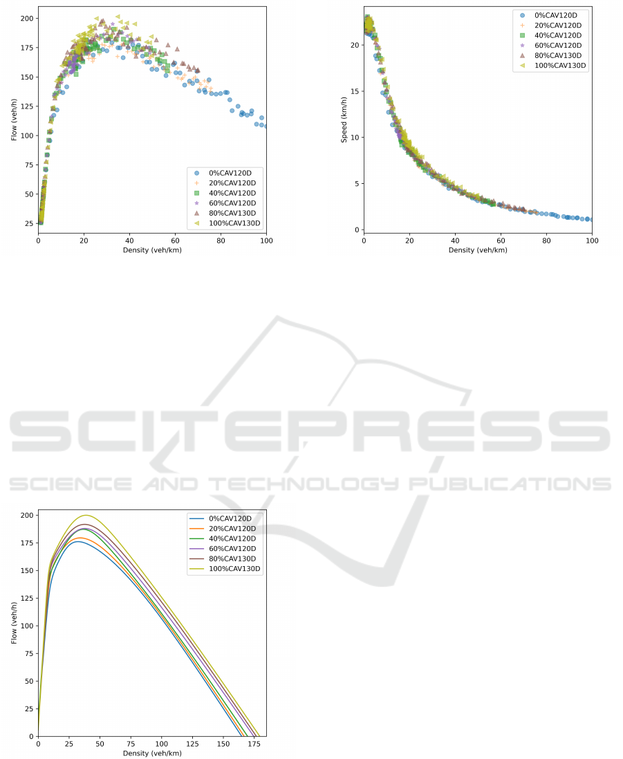
Figure 3: Flow density relationship.

of CAVs increases from 0% to 100%, the maximum

trafﬁc ﬂow of the Dublin road network increases by

approximately 13.6%, from around 176 vehicles/h to

200 vehicles/h. The critical density varies between

30 to 40 vehicles/km, as similarly happens in Tym-

pakianaki et al. (2022). This work estimated the crit-

ical densities for different scenarios to calculate the

congestion duration (∆) and over-saturation degree

(S%). With the available data, MFD curves are ﬁt-

ted for each scenario to ﬁnd the exact critical density

and maximum ﬂow. As shown in Fig. 4, the curves

are plotted with an upper bound MFD (uMFD) intro-

duced by Amb

uhl et al. (2020).

Figure 4: Fitted ﬂow density relationship.

4.2 Speed

In Fig. 5, the empirical MFD relationships between

network average speed and density have been pre-

Figure 5: Speed density relationship.

sented for each performed scenario. The scenarios in

Fig. 5 are the same as those in Fig. 3. For the same

vehicle density, scenarios with higher CAVs penetra-

tion have relatively higher average speeds. This is in

line with the simulation results of Barcelona’s central

business district in Tympakianaki et al. (2022).

4.3 Simulation State

SUMO provides a statistical output that reveals over-

all information about the simulation. Table 3 shows

a part of the statistic results, the critical density, and

the maximum ﬂow of different scenarios. As shown

in Table 3, the variable Vehicles means how many ve-

hicles are loaded and ﬁnished their trips. The speed

(in kilometers per hour) is the average trip speed. Du-

ration (in second) is the average trip duration. Wait-

ing time (in seconds) is the average time each vehicle

spends standing because of congestion or red trafﬁc

light. Time loss (in seconds), including waiting time,

is the average time lost due to driving slower than the

desired speed. Route length (in meters) is the average

route length. Critical density and maximum ﬂow were

obtained from the ﬁtted MFD curves. Comparing the

average speed of different scenarios with the same

travel demand, we can ﬁnd that the average speed in-

crease with a higher percentage of CAVs. From the

time loss and waiting time, one can conclude that it

is the waiting time that contributes much more to the

delay than the slower velocity. The maximum ﬂow is

increasing with a higher CAV penetration rate. The

maximum ﬂow of the network increased by 13.55%

with a 100% of CAV penetration rate. The improve-

ments in critical density and the maximum ﬂow have

a similar trend.

VEHITS 2023 - 9th International Conference on Vehicle Technology and Intelligent Transport Systems

382

Table 3: Simulation state.

Scenario Vehicles Speed Duration Waiting time Time loss Route length Critical density Maximum Flow

0%CAV120D 501597 10.48 15986.35 13834.23 15331.16 5782.56 32.25 176.01

20%CAV120D 501597 14.04 5515.88 4401.23 5070.34 4478.76 34.02 (+5.49%) 179.39 (+1.92%)

40%CAV120D 501597 16.34 2718.95 2054.61 2397.55 3317.37 36.58 (+13.43%) 187.15 (+6.33%)

60%CAV120D 501597 17.50 1901.73 1382.55 1621.13 2927.44 37.75 (+17.05%) 187.90 (+6.76%)

80%CAV120D 501597 20.81 599.33 306.51 397.68 2138.77 - -

100%CAV120D 501597 21.85 482.1 224.89 293.78 2015.42 - -

80%CAV130D 543396 15.37 4108.37 3326.23 3707.46 4086.4 37.56 (+16.47%) 191.62 (+8.87%)

100%CAV130D 543396 16.92 2141.14 1630.65 1838.31 3153.62 38.74 (+20.12%) 199..86 (+13.55%)

4.4 Congestion Duration and Roadway

Over-Saturation Degree

From Table 4, one can evaluate that in the case of

100% or even 110% of the original demand, all HDVs

scenarios have already had considerable congestion.

However, congestion does not occur yet in other sim-

ulated scenarios. This shows that the introduction of

CAVs alleviates trafﬁc congestion. When one looks

at the 120% of the original demand, the higher the

CAV penetration rate, the smaller the congestion du-

ration and over-saturated degree. Moreover, when

the CAV penetration rate is higher than 80%, one

will not observe over-congestion. The demand is in-

creased proportionally to observe the congestion in

80% and 100% CAV scenarios. When the demand

is increased to 130% of the original demand, conges-

tion appears in these two scenarios. When the de-

mand is increased to 130%, the 80% CAV penetra-

tion scenario have slightly heavier congestion than all

HDV scenario with the original demand. Moreover,

the full CAV scenario has lighter congestion than all

HDV with the original demand scenario.

Table 4: ∆ and S% for different scenarios.

Scenario 100% Demand 110% Demand 120% Demand 130% Demand

s% ∆ s% ∆ s% ∆ s% ∆

0%CAV 128.67 940 269 2290 306.32 3220 - -

20%CAV -63.22 0 -9.6 0 162.05 1700 - -

40%CAV -71.67 0 -52.72 0 73.92 880 - -

60%CAV -73.13 0 -63.69 0 44.21 600 - -

80%CAV -74.66 0 -66.39 0 -42.52 0 118.24 1300

100%CAV -78.43 0 -71.13 0 -58.03 0 52.67 680

When comparing the increase in maximum ﬂows

and demands, one may see that even if the maximum

ﬂow is increased only by 13.55%, the proportionally

increased demand that the road network can carry can

increase by more than 30%. This is because that trip

demand varies during the simulation.

Through Fig. 6, one can intuitively observe traf-

ﬁc improvement with different CAV penetration rates.

Fig. 6 shows the accumulated vehicle density changes

during each simulation. The critical density shown

in the ﬁgure is the critical density of the full HDV

scenario. The demand of the illustrated scenarios is

120% of the original demand. The simulation without

Figure 6: Vehicle density changes during the simulation.

CAVs lasts more than 70 hours to ﬁnish. The running

time of other scenarios is obviously shorter. There-

fore, a low CAVs penetration rate, such as 20%, may

contribute much to reducing simulation time.

5 CONCLUSIONS

This paper investigated the impacts of different CAV

penetration rates on the urban road network. The

CAVs have been assumed to have shorter time head-

way, less speed deviation, and better lane-changing

cooperation. Dublin city center was selected as the ur-

ban network for this research. The MFDs were used

to illustrate the impacts on the road network’s max-

imum ﬂow and average speed with different CAVs

penetration. This work veriﬁed that a road network

could have less scattered MFDs, even if the traf-

ﬁc ﬂow is distributed heterogeneously in a simula-

tion way. Congestion duration and roadway over-

saturation degree were introduced to show the ability

of different CAVs penetration to deal with the over-

congested situation. As detailed in section 4, 20 sim-

ulations with different CAV penetration rates and de-

mands had been run.

Simulation results show that the application of

CAVs beneﬁts the maximum achieved ﬂow of the ur-

ban road network. This conclusion is consistent with

previous researches that had demonstrated the ben-

eﬁts of CAVs on urban trafﬁc (Tympakianaki et al.,

2022; Mavromatis et al., 2020). As shown in the re-

Impacts of Connected Automated Vehicles on Large Urban Road Network

383

sults section, the maximum ﬂow of 100% CAVs pene-

tration rate increased by approximately 13.55% com-

pared with the all HDVs scenario. Moreover, the im-

provements in critical density for different scenarios

have a similar trend with the maximum ﬂow improve-

ments. In terms of congestion level, even a low CAV

penetration rate may greatly improve the trafﬁc con-

dition. Table 4 shows that 20% of CAVs penetration

rate eliminates the congestion in the original demand

and 110% demand scenarios. In the 120% demand

scenario, 20% CAVs greatly reduce trafﬁc conges-

tion level. Last but not least, when the CAV pene-

tration rate rises from 0% to 100%, the increase in

the proportional demand the network can carry under

the same congestion degree is much more signiﬁcant

than the increase in the maximum ﬂow. In this work,

the increase in the proportional demand is more than

two times the increase in maximum ﬂow. This is due

to the introduction of CAVs reducing the congestion

level and making the congestion dissipate faster. At

the same time, a daily demand rather than a constant

demand enlarges the advantage.

However, there is a limitation in this study. The

trafﬁc ﬂow is heterogeneously distributed, which

means the transportation system still has untapped po-

tential. The capacity of the trafﬁc system will be more

fully utilized if a control algorithm is used to control

the distribution of trafﬁc as homogeneously as possi-

ble, which we leave as future work.

ACKNOWLEDGEMENTS

The research reported in this paper is part of the

project Prin 2020 DigiT-CCAM-Digital Twins per

la Mobilit

a Cooperativa, Connessa e Automatizzata

(project no. 2020Z9HEMJ) funded by the Italian

Ministry of the University and the Research.

REFERENCES

Amb

uhl, L., Loder, A., Bliemer, M. C., Menendez, M., and

Axhausen, K. W. (2020). A functional form with a

physical meaning for the macroscopic fundamental di-

agram. Transportation Research Part B: Methodolog-

ical, 137:119–132.

Chen, D., Ahn, S., Chitturi, M., and Noyce, D. A. (2017).

Towards vehicle automation: Roadway capacity for-

mulation for trafﬁc mixed with regular and automated

vehicles. Transportation research part B: method-

ological, 100:196–221.

Daganzo, C. F. (2007). Urban gridlock: Macroscopic mod-

eling and mitigation approaches. Transportation Re-

search Part B: Methodological, 41(1):49–62.

Geroliminis, N. and Daganzo, C. F. (2008). Existence

of urban-scale macroscopic fundamental diagrams:

Some experimental ﬁndings. Transportation Research

Part B: Methodological, 42(9):759–770.

Geroliminis, N. and Sun, J. (2011). Properties of a well-

deﬁned macroscopic fundamental diagram for urban

trafﬁc. Transportation Research Part B: Methodolog-

ical, 45(3):605–617.

Ghiasi, A., Hussain, O., Qian, Z. S., and Li, X. (2017).

A mixed trafﬁc capacity analysis and lane manage-

ment model for connected automated vehicles: A

markov chain method. Transportation Research Part

B: Methodological, 106:266–292.

Godfrey, J. (1969). The mechanism of a road network. Traf-

ﬁc Engineering & Control, 8(8).

Goodall, N. J., Smith, B. L., and Park, B. (2013). Trafﬁc

signal control with connected vehicles. Transporta-

tion Research Record, 2381(1):65–72.

eriau, M. and Dusparic, I. (2020). Quantifying the im-

pact of connected and autonomous vehicles on trafﬁc

efﬁciency and safety in mixed trafﬁc. In 2020 IEEE

23rd International Conference on Intelligent Trans-

portation Systems (ITSC), pages 1–8. IEEE.

Herman, R. and Prigogine, I. (1979). A two-ﬂuid approach

to town trafﬁc. Science, 204(4389):148–151.

Hu, G., Lu, W., Whalin, R. W., Wang, F., and Kwembe,

T. A. (2021). Analytical approximation for macro-

scopic fundamental diagram of urban corridor with

mixed human and connected and autonomous trafﬁc.

IET Intelligent Transport Systems, 15(2):261–272.

Liu, H., Kan, X., Shladover, S. E., Lu, X.-Y., and Ferlis,

R. E. (2018). Impact of cooperative adaptive cruise

control on multilane freeway merge capacity. Journal

of Intelligent Transportation Systems, 22(3):263–275.

Loder, A., Amb

uhl, L., Menendez, M., and Axhausen,

K. W. (2019). Understanding trafﬁc capacity of urban

networks. Scientiﬁc reports, 9(1):1–10.

Lopez, P. A., Behrisch, M., Bieker-Walz, L., Erdmann, J.,

otter

od, Y.-P., Hilbrich, R., L

ucken, L., Rummel,

J., Wagner, P., and Wießner, E. (2018). Microscopic

trafﬁc simulation using SUMO. In 2018 21st inter-

national conference on intelligent transportation sys-

tems (ITSC), pages 2575–2582. IEEE.

Lu, Q., Tettamanti, T., H

orcher, D., and Varga, I. (2020).

The impact of autonomous vehicles on urban trafﬁc

network capacity: an experimental analysis by mi-

croscopic trafﬁc simulation. Transportation Letters,

12(8):540–549.

ucken, L., Mintsis, E., Kallirroi, N. P., Alms, R., Fl

otter

od,

Y.-P., and Koutras, D. (2019). From automated to

manual - modeling control transitions with SUMO.

In Weber, M., Bieker-Walz, L., Hilbrich, R., and

Behrisch, M., editors, SUMO User Conference 2019,

volume 62 of EPiC Series in Computing, pages 124–

144. EasyChair.

Mahmud, S. S., Ferreira, L., Hoque, M. S., and Tavassoli,

A. (2017). Application of proximal surrogate indica-

tors for safety evaluation: A review of recent develop-

ments and research needs. IATSS research, 41(4):153–

163.

VEHITS 2023 - 9th International Conference on Vehicle Technology and Intelligent Transport Systems

384

Maske, H., Chu, T., and Kalabi

c, U. (2019). Large-

scale trafﬁc control using autonomous vehicles and

decentralized deep reinforcement learning. In 2019

IEEE Intelligent Transportation Systems Conference

(ITSC), pages 3816–3821. IEEE.

Mavromatis, I., Tassi, A., Piechocki, R. J., and Sooriyaban-

dara, M. (2020). On urban trafﬁc ﬂow beneﬁts of con-

nected and automated vehicles. In 2020 IEEE 91st

Vehicular Technology Conference (VTC2020-Spring),

pages 1–7. IEEE.

Mersky, A. C. and Samaras, C. (2016). Fuel economy test-

ing of autonomous vehicles. Transportation Research

Part C: Emerging Technologies, 65:31–48.

Milan

es, V. and Shladover, S. E. (2014). Modeling coopera-

tive and autonomous adaptive cruise control dynamic

responses using experimental data. Transportation

Research Part C: Emerging Technologies, 48:285–

300.

Papadoulis, A., Quddus, M., and Imprialou, M. (2019).

Evaluating the safety impact of connected and au-

tonomous vehicles on motorways. Accident Analysis

& Prevention, 124:12–22.

Raju, N. and Farah, H. (2021). Evolution of trafﬁc mi-

crosimulation and its use for modeling connected and

automated vehicles. Journal of Advanced Transporta-

tion, 2021:1–29.

Shi, X. and Li, X. (2021). Constructing a fundamen-

tal diagram for trafﬁc ﬂow with automated vehicles:

Methodology and demonstration. Transportation Re-

search Part B: Methodological, 150:279–292.

Treiber, M., Hennecke, A., and Helbing, D. (2000). Con-

gested trafﬁc states in empirical observations and mi-

croscopic simulations. Physical review E, 62(2):1805.

Treiber, M. and Kesting, A. (2013). Trafﬁc ﬂow dynamics.

Trafﬁc Flow Dynamics: Data, Models and Simulation,

Springer-Verlag Berlin Heidelberg, pages 983–1000.

Tympakianaki, A., Nogues, L., Casas, J., Brackstone, M.,

Oikonomou, M. G., Vlahogianni, E. I., Djukic, T., and

Yannis, G. (2022). Autonomous vehicles in urban net-

works: A simulation-based assessment. Transporta-

tion Research Record, 2676(10):540–552.

Van Arem, B., Van Driel, C. J., and Visser, R. (2006).

The impact of cooperative adaptive cruise control on

trafﬁc-ﬂow characteristics. IEEE Transactions on in-

telligent transportation systems, 7(4):429–436.

Wang, M., Daamen, W., Hoogendoorn, S. P., and van Arem,

B. (2015). Cooperative car-following control: Dis-

tributed algorithm and impact on moving jam features.

IEEE Transactions on Intelligent Transportation Sys-

tems, 17(5):1459–1471.

Xie, H., Tanin, E., Karunasekera, S., Qi, J., Zhang, R.,

Kulik, L., and Ramamohanarao, K. (2019). Quan-

tifying the impact of autonomous vehicles using mi-

croscopic simulations. In Proceedings of the 12th

ACM SIGSPATIAL International Workshop on Com-

putational Transportation Science, pages 1–10.

Xie, Y., Zhang, H., Gartner, N. H., and Arsava, T. (2017).

Collaborative merging strategy for freeway ramp op-

erations in a connected and autonomous vehicles en-

vironment. Journal of Intelligent Transportation Sys-

tems, 21(2):136–147.

Ye, L. and Yamamoto, T. (2018). Modeling connected and

autonomous vehicles in heterogeneous trafﬁc ﬂow.

Physica A: Statistical Mechanics and its Applications,

490:269–277.

Impacts of Connected Automated Vehicles on Large Urban Road Network

385