Consensus Simulator for Organisational Structures
Johannes S. Vorster
1 a
and Louise Leenen
1,2 b
1
Department of Computer Science, University of Western Cape, South Africa
2
CAIR, South Africa
Keywords:
Consensus, Consensus Simulation, Stochastic Simulation, Synchronization.
Abstract:
In this paper we present a new simulator to investigate consensus within organisations, based on organisational
structure, team dynamics, and artefacts. We model agents who can interact with each other and with artefacts,
as well as the mathematical models that govern agent behaviour. We show that for a fixed problem size, there
is a maximum time within which all agents will reach consensus, independent of number of agents. We present
the results from simulating wide ranges of problem sizes and agent group sizes and report on two significant
statistics; the time to reach consensus and the effort to reach consensus. The time to reach consensus has
implications for project delivery timelines, and the effort relates to project economics.
1 INTRODUCTION
The past two decades have seen debates on shifts in
organisational structures and project delivery method-
ologies. These debates originated with technology
companies that needed to cope with three factors,
namely, changes in technology, changes in competitor
position, and fast shifting customer demands. Often
quoted examples of such changes are shifts in team
structure (Reagans et al., 2016), shifts from vertical
to more horizontal organisations (Keupp et al., 2012),
and organisational structures that resemble network-
like forms (Chang and Harrington, 2000). The out-
comes seem to be leaning towards the conclusion that
more horizontal organisational structures and better
connected open-network structures create better eco-
nomic value in the form of faster delivery and less
resources (time and material) spent on projects and
thus deliver better returns on investments (Will et al.,
2019). Project complexity and the ability to find con-
sensus on approaches and solutions have been identi-
fied and studied as key reasons why large projects fail
(Kian et al., 2016).
Will et al. (2019) studied how organisational
structure affect the economics of accepting risky
projects. In particular, they study the effect of the
selection process and the economic impact of organi-
sational structure on risky and innovation projects se-
lection. They argue that the selection of innovations
to pursue from an available portfolio is not only de-
a
https://orcid.org/0000-0001-6452-4186
b
https://orcid.org/0000-0002-9212-550X
pendent on the team’s evaluation skills, but also on
the organisational structure. They approach the topic
with a purely mathematical model. They showed
that, for example, hybrid organisational architectures
tend to have side effects in terms of handling er-
rors. S
´
aenz-Royo and Lozano-Rojo (2023) conducted
similar simulated structures to investigate innovation
project selection.
Human consensus in formal settings, such as pre-
diction of economic outcomes, are often conducted
by using Delphi processes where a group is led to
consensus though repeated rounds of providing views
anonymously. There are other methods to study con-
sensus, qualitative studies of social networks and con-
sensus emergence within these networks (Carter et al.,
2015; Jones and Shah, 2016). A second approach
is to conduct detailed interviews and study the phe-
nomenon qualitatively (Rosell
´
o et al., 2010). A third
approach is to study consensus through computational
models (Yan et al., 2017). This paper employs the last
approach, but also incorporates aspects of Delphi de-
cision making.
In this paper we report on the implementation of
a simulator for the study of organisational structures,
team dynamics and economic implications. We
observe that project implementations are a series
of consensus-seeking processes, where teams must
agree on vision, scope, requirements, architecture,
design, implementation details, construction de-
cisions, security controls, testing, quality control
measures, and so on.
Vorster, J. and Leenen, L.
Consensus Simulator for Organisational Structures.
DOI: 10.5220/0012017400003546
In Proceedings of the 13th International Conference on Simulation and Modeling Methodologies, Technologies and Applications (SIMULTECH 2023), pages 15-26
ISBN: 978-989-758-668-2; ISSN: 2184-2841
Copyright
c
 2023 by SCITEPRESS – Science and Technology Publications, Lda. Under CC license (CC BY-NC-ND 4.0)
15

We follow a stochastic agent-based modelling ap-
proach, where connections between agents simulate
organisational structure and communications chan-
nels as well as access to artefacts. Agents have prior
opinions about topics, which can be modelled using
various statistical distributions. The model simulates
the best-case consensus effort and time for the config-
uration of organisational architecture and team struc-
ture to reach consensus.
An aspect important to this simulation is that
agents manage their time by keeping diaries and can-
not have multiple meetings at the same time. Meet-
ings are the means to settle differences in views and
agents are restricted in the number of topics that can
be discussed per meeting.
We provide details for the model and the simula-
tor, as well as initial results regarding the impact of
artefacts on consensus seeking processes and organi-
sational efficiency.
In the next section the model is described, which
is followed in section three with a mathematical treat-
ment of the model. In section four the results from
simulating various scenarios are presented and dis-
cussed.
2 MODEL DESCRIPTION
In this section we discuss the construction of our
model of consensus and the simulator that was built to
implement that model. Topics covered are organisa-
tional architecture, the graph theory model, consensus
measures, artefacts, agent actions, diaries, and effort
& time measures.
2.1 Variations in Organisational
Architecture
The two extreme forms of organisational architectures
are Polyarchies (Figure 1) and Hierarchies (Figure 2)
(see Will et al. (2019) for a discussion). Hybrid or-
ganisations (Figure 3) are somewhere between these
two architectures.
2.1.1 Polyarchical Organisations
In polyarchical organisations (Figure 1) the agents
are peers with the same capabilities, organisational
power, and connectedness. Agents have a view of ev-
ery other agent’s position on topics and they can take
actions to reach consensus with each other. If agents
share artefacts such as plans or requirements, they can
simultaneously work on parts of the artefacts.
2.1.2 Hierarchical Organisations
In the case of a hierarchical organisation (Figure 2),
managers on different levels also differ in decision-
making powers. Managers on the same level have
different executive functions. In this organisational
structure, information flow and consensus-seeking
processes must follow the hierarchical rules in that
subordinates convey information only up and down
the ’chain of command’ and thus this hierarchy also
places constraints on the way consensus-seeking tasks
such as meetings are conducted. An agent can only
organise a meeting with peers, subordinates or their
manager.
In such an organisation, the top-level managers
may provide a project vision, which is translated into
a requirements specification by one group, an archi-
tecture by a second group, and a detailed delivery plan
by a third group. The artefacts that are finally deliv-
ered (the software system in the case of such a project,
or the road system if that was the project) can be mea-
sured against the expectation (the vision) of the top-
level manager, and against other planning artefacts.
2.1.3 Hybrid Organisations
The hybrid organisational architecture (Figure 3) is
a combination of polyarchical and hierarchical struc-
tures (Christensen and Knudsen, 2010; Will et al.,
2019). The organisation has a hierarchy, but agents
are not forced to communicate and structure decisions
within that hierarchy and can communicate with peers
in other teams or departments. This facilitates consen-
sus processes to work both vertically and horizontally
(Young-Hyman, 2017).
2.2 Graph Theory Preliminaries
Agents will be denoted ν
i
for the i
th
agent from a set
of N agents. In classical agent consensus theory the
agents are represented as vertices in a graph and the
edges represent the connections between agents (e.g.
Wei et al. (2021)). We extend those definitions to in-
clude artefacts.
Let G = (V,ε,∆) be a directed graph, where V =
V
ν
∪V
A
the set of vertices with V
ν
= {ν
i
|i ∈ I
ν
=
{1,2,. .., N}} the vertices that represent N agents and
V
A
= {c
p
|p ∈ I
A
= {1 + N,. .., M + N}} the vertices
that represent M artefacts. The index set over V is
then I = I
ν
∪I
A
.
The set of edges is represented by ε ⊆V ×V . Then
e
i j
∈ε, i, j ∈I, represent an edge of G that correspond
to an interaction. The element δ
i j
in the adjacency
matrix ∆ = [δ
i j
] correspond to e
i j
, and δ
i j
is positive
if and only if e
i j
∈ ε, otherwise δ
i j
= 0.
SIMULTECH 2023 - 13th International Conference on Simulation and Modeling Methodologies, Technologies and Applications
16

N
N −1
···
1
2
3
4
5
Figure 1: Polyarchy.
A0
B0
.
.
.
.
B1
.
.
.
.
B2
.
.
.
.
B3
.
.
.
.
Figure 2: Hierarchical.
A0
B0
.
.
.
.
B1
.
.
.
.
B2
.
.
.
.
B3
.
.
.
.
Figure 3: Hybrid.
If ν
i
,ν
j
∈V then information can flow from ν
i
to
ν
j
if δ
i j
> 0. A graph is directed if, for some i, j ∈ I
δ
i j
> 0 but δ
ji
= 0. That is, ν
i
can interact with ν
j
,
but ν
j
cannot interact with ν
i
. Otherwise it is undi-
rected. Artefacts cannot interact with each other and
thus δ
pq
= 0, ∀p,q ∈ I
c
.
The numeric value δ
i j
can represent some charac-
teristic of the interaction such as the amount of infor-
mation transmitted, the bandwidth, or the probability
of successful communication. In the work presented
here
δ
i j
=
(
1 e
i j
∈ ε
a
0 otherwise.
2.3 Topics, Views, and Artefacts
An agent ν
i
∈ V
ν
can have a view (synonymous to
opinion and belief) on a number of topics. If k is an
index number to the topics, k ∈ I
B
= {1, 2,.. .,B
max
},
then b
k
i
denote the view of agent i on topic k. Top-
ics are independent of each other since each topic is
about something specific. Topic k is the same topic
for all agents, although each agent can have a differ-
ent view on that topic. Thus b
k
i
, agent i’s view on topic
k, can be compared with b
k
j
, agent j ’s view on topic k.
However, b
k
i
cannot be compared with b
m
j
, if k ̸= m.
An artefact represents a set of codified (written
down, or captured in some other way) views on top-
ics. Topic k is codified in artefact p by c
k
p
. There
may be many artefacts c
p
, p ∈ I
c
and many topics
k ∈ I
C
= {1, ... ,C
max
}. Since c
k
p
is the codifica-
tion of topic k, it is possible to compare c
k
p
with b
k
i
,
k ≤ min(B
max
,C
max
). Note that C
max
and B
max
could
be different. That is, the artefact could cover more
topics (C
max
> B
max
), or less, or the same number of
topics than what agents may have views about.
2.4 Modelling Consensus
Next we address the question of how to compare top-
ics with each other. We are interested in a measure
that reflect an agents’ level of consensus with the
other agents in its network as well as an overall mea-
sure of group consensus.
In agent-based modelling, consensus between an
agent and the rest of its connected group on a specific
topic k is often expressed as the sum of differences
between agent i and all other agents j, (see e.g. Wei
et al. (2021)),
u
k
i
= −
N
∑
j=1
δ
i j
(b
k
i
−b
k
j
), i ∈ {1,2,. ..,N}.
This definition computes the average difference,
and can be negative. This way of measuring consen-
sus has the aim to indicate to the agent in what di-
rection (positive or negative) the group average is lo-
cated. The agents will then modify their view to move
towards the group average.
However, this definition of consensus does not
suite us here, since it leads to the strange situation
where if b
k
1
= 0, b
k
2
= 5, and b
k
3
= 10, then u
k
2
=
(b
k
2
−b
k
1
) + (b
k
2
−b
k
3
) = 0 which seem to imply that it
is in consensus with the other agents whereas it only
holds the average view.
In human consensus processes, the most famous
of which is the Delphi process, consensus can be mea-
sured in may ways, one of which is the sum of a pair-
wise comparison of views between agents (see e.g.
Birko et al. (2015) for the many ways to measure con-
sensus in Delphi processes).
We are interested in how far away the group of
agents are from a state of consensus, and thus opt for
the sum of absolute differences as the consensus mea-
sure, and sum over all pairwise agents and all topics.
A full justification and comparison with other alter-
natives is beyond the scope of this paper. We thus
opt for a measure that is a combination of consensus
measures from Delphi (pairwise comparison of con-
sensus) and agent-based modelling. We use absolute
differences since we want to capture how far agents
are from consensus. Furthermore, we include arte-
facts in the evaluation and measure how well agents
are in consensus with the artefacts.
We used the approach of defining a measure of
consensus for agents with each other (i, j ∈ I
ν
) and
Consensus Simulator for Organisational Structures
17

agents with artefacts (i ∈ I
ν
, p ∈ I
A
) as
u
k
i j
= δ
i j
|b
k
i
−b
k
j
| and u
k
ip
= δ
ip
|b
k
i
−c
k
p
|
which leads to an overall measure of consensus for an
agent i with agents and artefacts it has contact with as
u
k
i
=
∑
j∈I
ν
δ
i j
|b
k
i
−b
k
j
|+
∑
p∈I
A
δ
ip
|b
k
i
−c
k
p
|. (1)
That is, the level of consensus that an agent i has rel-
ative to the rest of the group on a topic k, is the sum
of absolute differences between that view b
k
i
and the
views on the same topic for all other agents, b
k
j
that it
is connected to, (δ
i j
> 0), as well as the same measure
for that topic in all artefacts, c
k
p
, that it has access to.
The consensus of an agent with its group of con-
nected agents and artefacts over all topics is given by
u
i
=
∑
j∈I
ν
B
max
∑
k=1
δ
i j
|b
k
i
−b
k
j
|+
∑
p∈I
A
MX
∑
k=1
δ
ip
|b
k
i
−c
k
p
|, (2)
where MX = min(B
max
,C
max
), see section 2.3.
The overall consensus on a specific topic k can
also be defined using (1) as
u
k
=
∑
i∈I
ν
∑
j∈I
ν
δ
i j
|b
k
i
−b
k
j
|+
∑
i∈I
ν
∑
p∈I
A
δ
ip
|b
k
i
−c
k
p
|. (3)
Finally, we can now define an overall level of con-
sensus over all agents, that is, an overall level of con-
sensus for the group as
u =
∑
i∈I
ν
u
i
. (4)
As will be shown shortly in section 3.3, the con-
sensus follows an exponential decrease. Therefore,
we also represent the consensus as the natural log of
u
S
u
= ln(u). (5)
This measure of consensus is more descriptive and
insightful than using u, as will be discussed in the re-
sults section, 4.2.
We want to be able to model the situation where
agents may believe that they are in consensus with
another agent or artefact, but in fact are not. This is
a common situation, where people believe they are
in agreement, but subsequent more detailed analysis
shows that they are in fact not in agreement. This is
achieved by introducing a consensus threshold, κ. If
the absolute difference in views on a topic is within
this threshold, the agents will consider that topic as
synchronized and no further discussions or actions
will involve that topic. Consensus is reached when
u
k
i j
= δ
i j
|b
k
i
−b
k
j
| ≤ κ. That is, the agents will believe
that consensus is not reached if u
k
i j
> κ and will take
further actions to achieve consensus on topic k with
agent j. The same holds for artefact consensus and if
u
k
ip
= |b
k
i
−c
k
p
| ≤ κ the agent will consider that it is in
consensus with artefact p on topic k.
Consider an example of the consequence of the
introduction of κ. The project sponsor generates a
project vision document where his actual vision dif-
fers from what is documented by κ. The business
analyst reads this document, again with a κ margin,
which now creates a 2 ·κ difference between what
the analyst understands and what the project sponsor
meant. In this way, a chain of agents and artefacts can
create an ever increasing ’error’ between the original
meaning and what is understood later in the chain.
In all the simulations conducted and reported on
later κ = 2.
2.5 Agent Actions and Diaries
Artefacts could be assigned to every member of the
group. The assignment also specifies the actions that
each agent is allowed to take on its assigned artefact,
namely writing to the artefact, reading from the arte-
fact, or both. One group of agents may be responsible
for writing an artefact, for example project require-
ments, software source code, or the architecture doc-
ument for a new road network. While another group
may only read that artefact, for example the construc-
tion team can only read the architecture document and
cannot directly change it.
Agents can take only one action in a time interval.
At the beginning of the time interval, each agent (ν
i
)
constructs a plan which consists of all potential ac-
tions available. This plan consists of agents and arte-
facts that ν
i
has connections to, and that have topics
where consensus has not been reached. Therefore the
agent will identify all ν
j
, δ
i j
> 0, for which there ex-
ists a k so that |b
k
i
−b
k
j
| > κ. Similarly they will iden-
tify all artefacts c
p
, δ
ip
> 0 for which there exists a k
so that |b
k
i
−c
k
p
| > κ.
An agent selects at random from the set of actions
in its plan. These actions are:
• Meet with another agent, ν
j
. A meeting is
recorded in both agents’ diaries. A random num-
ber of topics, d, are discussed, where |b
k
i
−b
k
j
| >
κ, d ∈I
D
= {1, ... ,D
max
−1}with expected value
ˆ
d = D
max
/2. For every topic, k, discussed, one of
three outcomes is selected at random; (a) a com-
promised consensus where the new b
k
i
and b
k
j
are
set to the average of their values at the beginning
of the meeting, (b) ν
i
accepts the view of ν
j
by
setting b
k
i
= b
k
j
; or (c) ν
j
accepts the view of ν
i
by
setting b
k
j
= b
k
i
.
• Read an artefact p if an artefact is present and
SIMULTECH 2023 - 13th International Conference on Simulation and Modeling Methodologies, Technologies and Applications
18

the read action is allowed. The agent interacts
with the artefact and updates its own views on
a random number, d ∈ I
D
, of topics where con-
sensus has not been reached, by setting b
k
i
= c
k
p
,
k ≤ min(B
max
,C
max
).
• Write to artefact p if an artefact is present and
the write action is allowed. Here the agent im-
parts its views into the artefact, setting c
k
p
= b
k
i
for a random number of topics, d ∈ i
D
and k ≤
min(B
max
,C
max
).
• Do nothing. If an agent cannot construct a plan,
because it is in consensus with all agents in its
network and all artefacts it has access to, then it
will do nothing during that time interval.
The order in which agents take action is random-
ized at the beginning of each time interval. If an agent
(ν
j
) was involved in a meeting with another agent (ν
i
)
due to ν
i
taking an action earlier, then ν
j
was already
involved in an action this time interval and cannot take
a further action.
An agent’s diary captures the action it took in that
time interval. We use d
t
i
to represent the diary action
of ν
i
at time t. It is a historic record that can be anal-
ysed later to understand how productive an agent was
and other behavioural statistics. If ν
i
was the origi-
nator of a meeting, it is indicated with d
t
i
= ’O’. If
a meeting was attended, but ν
i
was not the originator,
then d
t
i
= ’m’. For the actions to read, write, or update
an artefact the diary entries are d
t
i
= ’r’, d
t
i
= ’w’, and
d
t
i
= ’u’ respectively. If the agent could not take any
action then d
t
i
= ’z’.
2.6 Effort, Time, and Productiveness
The effort, e
max
, to reach consensus is the sum of all
actions taken by all agents, that is
e
max
=
t
max
∑
t=1
N
∑
i=1
busy(d
t
i
), busy(d
t
i
) =
(
0 d
t
i
= ’z’
1 otherwise,
(6)
where t
max
is the total time it took to reach consensus.
Since each agent will always take some action if an
action is available, the simulation terminates at time
t
max
when d
t
i
= ’z’ ∀i ∈I
ν
. That is, when all agents no
longer takes any actions, the simulation stops. Both
e
max
and t
max
will be determined by simulation and
will differ on each stochastic simulation.
These two variables, i.e. the effort measured by
e
max
and time by t
max
, are the measures we are most
interested in. This paper started off by asserting that
all projects are consensus-seeking processes that can
complete successfully only if consensus is reached
through the various phases and deliverables of the
project. The effort can be translated into an economic
measure by noting that it measures agents’ time spent
on the project, and time multiplied by rate gives cost.
The overall time to complete the project (that is, cal-
endar time) also has economic implications if oppor-
tunity costs and Net Present Values are considered.
In subsequent work we want to establish the char-
acteristics of these two variables as a function of the
organisational structure, project delivery methodol-
ogy and even team dynamics. However, here we focus
on the simulator and the basic results using polyarchy
organisations as a benchmark for future work.
The configurations discussed in this paper is such
that the agents are almost fully engaged and produc-
tive. That is not the case in all configurations. Part
of what makes this interesting is that agents may be-
come very unproductive for large periods in specific
configurations. This may be the case where a sub-
set of agents are responsible for writing requirements
and another team is responsible for the implementa-
tion of those requirements. Initially the requirements
writing agents will be engaged in artefact writing ac-
tivities, but then they may be idle for a while while
other agents assimilate the requirements, followed by
a frenzy of activities as the agents try to resolve differ-
ences of views and reach consensus. These configu-
rations are not reported here, but form part of the long
term initiative we aim to report on in future papers.
3 MATHEMATICAL MODEL
PRELIMINARIES
This paper does not expand on the full mathemati-
cal model, since the main aim is to model complex
project configurations that may involve complexities
better handled with simulation. However, some of the
observed trends for polyarchies can be explained with
mathematical models and so we offer a non-rigorous
formalism here. Furthermore, if the simulation ad-
heres to the model, it acts as validation that the im-
plementation performs as expected and thus were im-
plemented correctly. This bolsters confidence in the
results produced by later simulations with more com-
plex configurations.
This section assumes no artefacts are present. A
group of N fully connected agents in a polyarchy will
be called an N-group. For example a group of 15 fully
connected agents will be called a 15-group.
3.1 Nomenclature Revisited
Agents (index set I
ν
) in an N-group has opinions
about B
max
topics (index set I
B
). An artefact contains
Consensus Simulator for Organisational Structures
19

C
max
codified topics (index set I
C
). The maximum
number of topics that can be discussed and concluded
per action is (D
max
−1), the minimum is one, the ex-
pected number (denoted with a hat) is
ˆ
d = D
max
/2. (7)
The topics, a total of B
max
, is fixed for a given
simulation and all agents within the group has B
max
topics
3.2 Initial Conditions
If f (x,t) is the distribution function for the agent
views (b
k
i
) at time t, then the expected value of the
mean absolute difference of the consensus measure
between the views of two agents |b
k
i
−b
k
j
| = u
k
i j
is
given by
ˆu
k
i j
(t) =
Z
∞
x=−∞
Z
∞
y=−∞
|x · f (x,t) −y · f (y,t)|
(8)
and thus, depending on the distribution,
ˆu
k
i j
(t) =









1
3
∆
b
Uniform(∆
b
)
2·σ
√
π
Normal(µ,σ)
1
λ
Exponential(λ)
3
2λ
Symmetrical Exponential(λ)
(9)
on topic k. Real world distributions of opin-
ions have been shown to have Uniform (Den Boon
and Van Meurs, 1991), Normal (Den Boon and
Van Meurs, 1991) and Exponential (Lang et al., 2018)
distributions, depending on the specifics of the topic.
We make the assumption that opinions are Normally
distributed for some topic so that ˆu
k
i j
=
2σ(t)
√
π
and σ(t)
is time-dependent since the distribution will change
over time.
At t=0 all agents are initialized with random views
per topic, b
k
i
∼ N (σ = 100), from the Normal distri-
bution.
The expected value for u
k
i j
(t = 0) in our simula-
tions with σ(0) = 100 is then
ˆu
k
i j
(0) =
200
√
π
. (10)
The group consensus measure, given ˆu
k
i j
(t), using (4),
is
ˆu(t) =
∑
i∈I
ν
∑
j∈I
ν
B
max
∑
k=1
ˆu
k
i j
(t) = B
max
N(N −1) ˆu
k
i j
(t) (11)
keeping in mind that u
k
ii
= 0. At t = 0
ˆu(0) =
∑
i∈I
ν
B
max
∑
k=1
ˆu
k
i
= B
max
N(N −1)
2σ(0)
√
π
. (12)
The simulation ends when |b
k
i
−b
k
j
| < κ, ∀i, j at
t = t
max
. The expected value of |b
k
i
−b
k
j
| is then κ/2
and thus
ˆu(t
max
) ≈
1
2
κB
max
N(N −1). (13)
3.3 Consensus Change
Agents decide randomly between one of three options
to resolve a topic with another agent (or an artefact)
as discussed in section 2.5. For option (a) both com-
promise to the mean value of their views, in option
(b) ν
i
adopts the position of ν
j
and option (c) is the
reverse. Each of these events happen with 1/3 chance
and the expected change in consensus due to each of
these events can be computed using expected values
from the Folded Normal distribution and summing us-
ing (4). The derivation is too lengthy to replicate here
and we only provide the result by case. For option
(a)
1
∆ ˆu
k
i j
(t)
(a)
= −
1
3
ˆu
k
i j
·2
h
(2
√
3 −3) + (2 −
√
3)N
i
(14)
for cases (b) and (c)
∆ ˆu
k
i j
(t)
(b,c)
= −
1
3
ˆu
k
i j
(t) ·2
(15)
so that for all three cases
∆ ˆu
k
i j
(t) = −
2
3
h
(2
√
3 −1) + (2 −
√
3)N
i
ˆu
k
i j
(t)
= −g
′
(N) · ˆu
k
i j
(t)
(16)
where
g
′
(N) =
2
3
h
(2
√
3 −1) + (2 −
√
3)N
i
(17)
This result is dependent on the choice of initial
distribution for b
k
i
, and consequently ˆu
k
i j
from (9).
Figure 4 shows the distribution of u
k
i j
= |b
k
i
−b
k
j
| as
well as its evolution for various time instances, col-
lected over many simulations. These graphs uses
a log-y scale, b
k
i
(t = 0) ∼ N (σ = 100), and thus
u
k
i j
(t = 0) has a Folded Normal distribution. The evo-
lution of the distribution of u
k
i j
causes the model pre-
sented by (16) to become less accurate in later time
1
Breadcrumbs to verify option (a) results: b
k
i
∼ σ
i
,
b
k
i
−b
k
j
∼ σ
i−j
=
√
2σ
i
, u
k
i j
= |b
k
i
−b
k
j
| is Folded-Normal,
thus u
k
i j
∼
q
2
π
·σ
i−j
= 2σ
i
/
√
π. Option (a): m =
b
k
i
+b
k
j
2
,
σ
m
= σ
(i+ j)/2
= σ
i
/
√
2, σ
m−i
=
q
σ
2
m
+ σ
2
i
=
p
3/2σ
i
,
|m −b
k
i
| ∼
p
2/π
p
3/2σ
i
. Now sum ∆u
k
= u
k
(t + 1) −
u
k
(t) using (4).
SIMULTECH 2023 - 13th International Conference on Simulation and Modeling Methodologies, Technologies and Applications
20

10
−6
10
−4
10
−2
%
t = 0
10
−6
10
−4
10
−2
%
t = 25
10
−6
10
−4
10
−2
%
t = 50
10
−6
10
−4
10
−2
%
t = 75
10
−6
10
−4
10
−2
%
t = 100
0 100 200 300 400
500 600
700
10
−6
10
−4
10
−2
u
k
i j
= |b
k
i
−b
k
j
|
%
t = 125
Figure 4: As the consensus process continues, the distri-
bution of differences in opinions, u
k
i j
= |b
k
i
−b
k
j
|, changes.
Data shown are from simulations with a 50-group, B
max
=
50 views on which to reach consensus, and b
k
i
(0) ∼ N (σ =
100).
steps. We do not see an easy way to build a model
that tracks this change in distribution. One approach
would be to introduce a sigmoid function to help cor-
rect for the change in distribution characteristics and
we leave that for future work.
The expected change in the consensus measure for
a single time interval at some time t, ∆t = 1, is then
the sum over all events, that is, through N/2 meet-
ings wherein an expected
ˆ
d topics are discussed per
meeting, leading to
∆ ˆu(t) =
N/2
∑
1
ˆ
d
∑
1
∆ ˆu
k
i j
(t)
= −
ˆ
d ·
N
2
·g
′
(N) · ˆu
k
i j
(t).
(18)
Substituting ˆu
k
i j
(t) from (11) gives
∆ ˆu(t) = −
ˆ
d ·N ·g
′
(N)
2 ·B
max
N(N −1)
· ˆu(t)
= −
ˆ
d
2B
max
g
′
(N)
N −1
· ˆu(t)
which can be written as
∆ ˆu(t) = −a
0
· ˆu(t),
a
0
=
ˆ
d
2B
max
·
g
′
(N)
N −1
=
ˆ
d
3B
max
·
(2
√
3 −1) + (2 −
√
3)N
N −1
(19)
where a
0
is now dependent on B
max
,
ˆ
d, and N, but
static for a simulation.
3.4 Consensus
The expected value for u , at t +1 is u(t + 1) = ˆu(t)+
∆ ˆu(t), which we can now compute by using ˆu(t) from
(11) and ∆ ˆu(t) from (19) to give
ˆu(t + 1) = (1 −a
0
) ˆu(t)
and thus
ˆu(t) = ˆu(0) ·(1 −a
0
)
t
.
(20)
3.5 Meeting Assumptions
The above equations that describe the measure of
consensus and consensus delta per time interval are
subject to the assumption that D
max
topics are avail-
able for discussion. However, as the simulation pro-
gresses, a time is reached when agents have reached a
level of consensus with other agents so that the num-
ber of topics available between an agent i and j is less
than D
max
.
At that time, the above equation is no longer valid
- at least in the sense that the number of topics that can
be discussed per meeting is no longer d ∈ I
D
, since
there are less than D
max
available topics to discuss.
That is, the expected number of topics discussed per
meeting,
ˆ
d starts to decrease, meetings are less effi-
cient, and ∆ ˆu(t) decreases as more and more topics
reach the consensus threshold κ.
As an example, it may be that agent i has five top-
ics to reach consensus on, but, each one is with a dif-
ferent agent. In that case the agent still needs to at-
tend five meetings one with each of the agents, but
each meeting can only discuss one topic, making the
meeting itself inefficient. This is not uncommon in
real life.
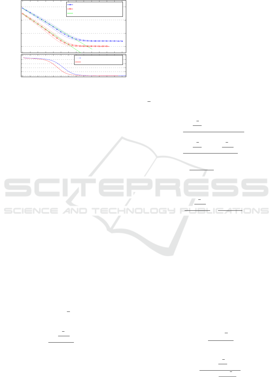
The situation is illustrated in Figure 5, which
shows the consensus trajectory (averaged over
n=25000 simulations) for a 20- and a 30-group. This
figure shows the model prediction using (20) and
ˆ
d = D
max
/2.
Consensus Simulator for Organisational Structures
21

8
10
12
14
Consensus Entropy (S
u
)
30-Group
20-Group
Initial model
ˆ
d = D
max
/2, Eq. (20)
0 10 20 30 40
50 60
70 80 90 100 110 120 130
1
2
3
4
5
6
Time
Average topics discussed
per meeting
Topics per meeting, 30-group
20-group
Figure 5: Later in the consensus process when the number
of topics that needs to be discussed between two agents are
less than the expectation,
ˆ
d = 5.5, the meetings become less
efficient. The consensus process is dominated by one-topic
meetings towards the end of the consensus process.
Two behavioural changes can be seen in Figure 5.
Firstly, the rate of change increases (graph drops be-
low predictive model) as the distribution of b
k
i
slowly
changes away from Normal, as shown in Figure 4.
Secondly, as the number of topics available to discuss
starts to drop below D
max
and thus
ˆ
d and ∆ ˆu(t) dimin-
ishes, the rate decreases and the graph turns almost
horizontal as meetings become less efficient. Figure 5
(bottom) shows that towards the end the consensus
process is dominated by one-topic meetings.
This is an interesting result since it provides fur-
ther insights into why project projected timelines are
often exceeded. The one-topics region is a significant
portion of overall project time and thus warrants fur-
ther study both theoretically, quantitatively and quali-
tatively.
3.6 Estimations
Due to this change in the effectiveness of meetings as
agents come closer to reaching consensus, it is dif-
ficult to find good estimators for t
max
and e
max
. An
approximation can be found by using (13) to estimate
ˆu at t
max
, substitute into (20) and solve for t
1
as the
first estimation of t
max
. Thus
ˆu(0) ·(1 −a
0
)
t
1
=
1
2
κB
max
N(N −1)
which leads to
t
1
≈
ln

√
πακ
4σ

ln(1 −a
0
)
, α = 1, (21)
where the subscript of t
1
indicates that this is a first
approximation, and α is a scaling factor. If we want
to compute t
1
to be the expected value at consensus,
then α = 1. We will shortly use α as a scaling factor
to indicate when the consensus process reaches a time
of low meeting efficiency, where there are much less
than
ˆ
d topics available for discussion.
As a second approximation, we compute t to reach
ακ for every topic and then do a second estimation
of time to reach the expected κ/2 by using
ˆ
d = 0.2.
Use the first approximation, t
1
, to estimate u(t
1
), and
finally solve for t
2
, the second estimate, in
ˆu(t
′
2
) ≈ˆu(t
1
) ·(1 −a
1
)
t
′
2
= ˆu(0) ·(1 −a
0
)
t
1
·(1 −a
1
)
t
′
2
(22)
where a
1
is a
0
(
ˆ
d = 0.2), and ˆu(t
′
2
) is limited by (13)
which leads to
1
2
κB
max
N(N −1) = ˆu(0) ·(1 −a
0
)
t
1
·(1 −a
1
)
t
′
2
(23)
and solving for t
′
2
,
t
′
2
=
ln

√
πκ
2σ

−t
1
·ln(1 −a
0
)
ln(1 −a
1
)
=
ln

√
πκ
2σ

−ln

√
πακ
2σ

ln(1 −a
1
)
= −
ln(α)
ln(1 −a
1
)
(24)
and finally the second estimator of t
max
is
t
2
=t
1
+t
′
2
=
ln

√
πακ
2σ

ln(1 −a
0
)
−
ln(α)
ln(1 −a
1
)
(25)
If we set α = 1 then t
2
= t
1
as expected. So that
α can be used to help scale the predictor for more
accurate estimates.
As a final remark on time and effort estimation.
Since the effort is a sum over all events where agents
are busy over the time t
max
as per (6), it implies
e
max
≤ N ·t
max
.
(26)
3.7 Maximum Time and Effort
An interesting consequence of (21) is that it places a
limit on the time to reach consensus no matter what
the group size. That is, for a fixed number of topics,
the time to reach consensus has an upper limit. Con-
sider (19) in the limit N → ∞,
lim
N→∞
a
0
=
(2 −
√
3)
ˆ
d
3B
max
so that (21) with α = 1 gives
lim
N→∞
t
1
=
ln

√
πκ
4σ

ln

1 −
(2−
√
3)
ˆ
d
3B
max

(27)
SIMULTECH 2023 - 13th International Conference on Simulation and Modeling Methodologies, Technologies and Applications
22

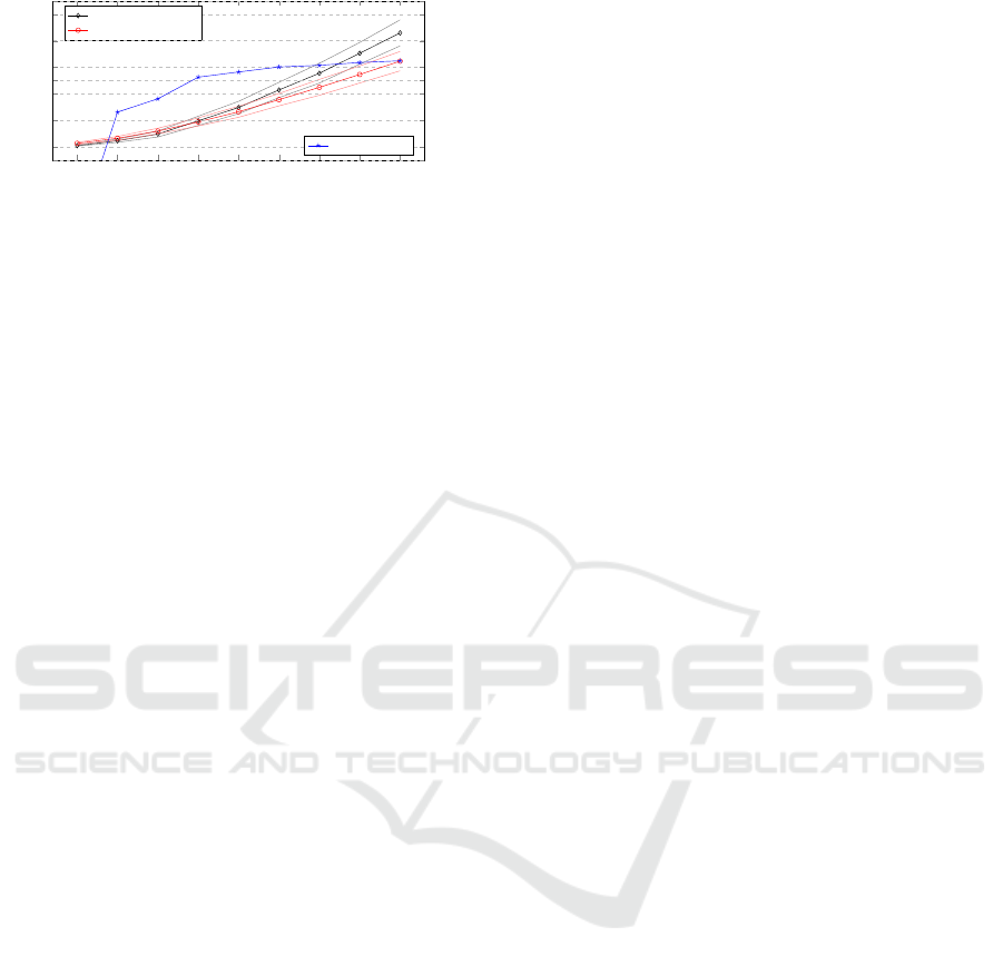
0
10
20
Time to reach consensus
100 topics
75 topics
50 topics
25 topics
2 4
6
8 10 12 14
16
18 20
0
100
200
300
Group-size
Effort to reach consensus
100 topics
75 topics
50 topics
25 topics
Figure 6: Time (Top) and effort (Bottom) to reach consen-
sus for small groups. Results were scaled relative to a 2-
group.
and if B
max
> 2
ˆ
d then
lim
N→∞
t
1
≈
3B
max
(2 −
√
3)
ˆ
d
·ln

4σ
√
πκ

.
(28)
The same is not true of the effort, e
max
, which, from
(26), grows at least linear with N and thus is un-
bounded even if t
max
has an upper limit.
ˆ
d has a physical limit in that no matter how fast
people talk in meetings, they can only discuss a lim-
ited number of topics in a given time. So that
ˆ
d is
fundamentally constrained. That is not the case with
B
max
which represent the complexity of the problem.
For large projects, such as the construction of a new
factory, or a new industrial complex, B
max
will be
very large.
3.8 Assumptions of Cooperation
Agents are fully cooperative, always reach consen-
sus on a topic at a meeting, and topics are indepen-
dent of each other. This is ideal world assumptions.
The results above, in particular the estimation of to-
tal effort (e
max
), total time to reach consensus (t
max
)
and the time to reach consensus independent of num-
ber of agents, (lim
N→∞
t
1
) are lower limits for real-
world consensus processes. That is, no matter how
hard real-world agents work, no matter how cooper-
ative they are, no matter how trivial the problem is
in terms of interdependencies, a project or task can-
not be completed in less time and with less effort than
what is given by these results.
In Figure 6 the graphs had been scaled so that the
time and effort for a 2-group is 1, and thus all other
numbers are relative to this 2-group. Using this as a
reference, and considering the results shown in this
figure, if a 2-group reaches consensus on a number
of topics in a certain time, then, a 6-group will take
about ten times longer, and the effort to reach con-
sensus for a 10-group will be about 100 times greater
than for a 2-group. In reality, where people may not
attend meetings, where they may not reach consen-
sus so easily, and where topics have interdependen-
cies that complicate the process of reaching consen-
sus, it will take even longer. The results presented
here should be considered a lower bound on the time
and effort to reach consensus due to the simplification
assumptions that were made.
4 MODELLING RESULTS
This section presents the results of experiments to
identify characteristics of this model through simu-
lations. The following topics are discussed; the ex-
perimental setup & data collection, the consensus &
entropy measures and their characteristics, the effect
on the number of topics, group size, and the presence
of artefacts on the time to reach consensus.
4.1 Experimental Setup and Data
Collection
The simulator we constructed is primarily for the in-
vestigation of team structure, organizational structure,
project delivery methodology, and other such organi-
sational aspects. However, this paper only reports on
the simulator’s design and results. We restrict the or-
ganizational structure to polyarchies and investigate
the effects of group size, number of topics, the pres-
ence of artefacts, and the number of facts that the arte-
facts contain. The primary measures used are the ef-
fort (e
max
) and the time to reach consensus (t
max
).
4.2 Consensus and Entropy
Figure 7 (Top) shows the consensus values u(t) over
time for twenty simulations of a group of ten agents
with δ
i j
= 1, ∀i, j ∈ {1,2,..., 10} and ten topics
(B
max
= 10). It also shows the average ¯u(t) over time
averaged over 25000 simulations. Each of these sim-
ulations reaches consensus as measured by the discus-
sion in section 2.6, but at different times.
Completing many such simulations allow the
computation of a histogram of t
max
. Figure 7 (Bot-
tom) shows this histogram (µ = 48.53, σ = 5.63,
n=25000) as well as a Normal (N ) distribution with
the same (µ, σ) parameters. The histogram is not
Normal. Visual inspection shows fat-tailed distribu-
Consensus Simulator for Organisational Structures
23

0
1
2
·10
4
Consensus (u)
Consensus for 20 simulations
Averaged Consensus
1-σ
Final consensus 1-σ
6
8
10
12
Consensus Entropy (S
u
)
Ln(Consensus) for 20 simulations
Ln(Consensus) averaged
1-σ
Final consensus 1-σ
0 10 20 30 40
50 60
70
0
1
2
3
4
5
6
7
8
9
Time (t
max
)
Count [%]
Histogram of t
max
LN (3.875,0.1157)
N (48.53,5.63)
0 10 20 30 40
50 60
70
1
2
3
4
5
6
7
8
9
Average topics discussed
per meeting
Topics per meeting (
¯
d)
Figure 7: (Top) Various simulations of the 10-group show-
ing the consensus measure over time. (Middle) The same
data as in top graph, but now using ln(consensus). (Bottom)
Histogram of the time it takes to reach consensus over many
such runs (µ = 48.53, σ = 5.63, n=25000) and Normal and
Lognormal fits to the histogram data.
tions and Kolmogorov-Smirnov (KS) and Shapiro-
Wilk (SW) tests fail. Figure 12 shows the histogram
for a 15-group together with a Gaussian distribution
for further edification.
Figure 7 (Middle) shows the same data as (Top)
but using the entropy measure. Under this measure
the entropy initially follows an approximately linear
decrease until very close to consensus. However, the
agents then take a significant time to resolve the small
differences in views to finally reach overall consen-
sus.
Figure 8 (Top) shows the consensus entropy (S
u
)
profiles averaged over n=25000 simulations for group
sizes of N ∈ {10, 20,.. .,50}. It also shows (Bot-
tom) the histograms for each of the distributions of
final consensus time (t
max
). As was already hinted
at, the distribution is not Normal and the best fit
we found was Lognormal LN , even so, it still fails
Kolmogorov-Smirnov tests.
4.3 Topics
To characterise the effect of the number of topics per
agent, B
max
, on the effort and time to reach consen-
sus a number of simulations were conducted for a
range of topics (10, 20, . . . 100, 200, . . . 500) keeping
6
8
10
12
14
Consensus Entropy (S
u
)
50-Group
40-Group
30-Group
20-Group
10-Group
Model (Eq. (20))
0 10 20 30 40
50 60
70 80 90 100 110 120 130 140
150 160
170
0
5
10
Time (t
max
)
Count [%]
Histogram
Lognormal fit
Figure 8: (Top) Group consensus entropy for group sizes of
10, 20, 30, 40, and 50, the bands indicate 1-σ, n=25000. Ev-
ery 5
th
symbol is shown to avoid symbol clutter. The solid
symbols indicate a 1-σ spread in t
max
. (Bottom) Histograms
for the group sizes, and the distribution mean indicated by
solid symbols and dotted lines.
0
1,000
2,000
Time to reach consensus (t
max
)
0
50
100
150
200
250
300
350
400
450 500
0
1
2
·10
4
Number of topics
Effort to reach consensus (e
max
)
Figure 9: The effect and time to reach consensus as a func-
tion of the number of topics.
the number of agents constant (N=10) in a fully con-
nected configuration, n=1 simulations per data point.
The results show an expected linear increase in ef-
fort and time to reach consensus, see Figure 9 which
shows the effort as a function of the number of topics.
It would be worthwhile, in future work, to explore the
effect of interdependent topics on the time to reach
consensus.
4.4 Group-Size
Next we report on the effect of groupsize on the ef-
fort and time to reach consensus. We vary the num-
ber of agents (N) per group, for group sizes N ∈
{5,10,. .., 100,200,. .., 1000}. For each such config-
uration we compute a number of stochastic simula-
tions to determine mean and standard deviations.
Figure 10 shows effort as as function of group size
SIMULTECH 2023 - 13th International Conference on Simulation and Modeling Methodologies, Technologies and Applications
24

0 10 20 30 40
50 60
70 80 90 100
0
2
4
6
8
·10
4
Group-size
Effort to reach consensus (e
max
)
100 topics
75 topics
50 topics
25 topics
10 topics
Figure 10: Effort to reach consensus for different group
sizes. The bands indicate 1-σ, n=20.
10
1
10
2
10
3
0
500
1,000
Group-size
Time to reach consensus (t
max
)
100 topics
75 topics
50 topics
Figure 11: Time to reach consensus for different group
sizes. The bands indicate 1-σ, n=10. The solid symbols on
the far right indicate maximum consensus time as N → ∞
as given by (27).
and for many different numbers of topics (B
max
). The
effort to reach consensus agree with (26) and is linear
in N for large N > 20.
The time to reach consensus as a function of group
size has a much more complex relationship as shown
in Figure 11. The predictive functions developed ear-
lier, (21) and (25), shows good approximations for
t
max
at least for larger group sizes as is shown in the
graph.
4.5 Artefacts
In this subsection we investigate the effects of intro-
ducing artefacts that capture views on the range of
topics. We are interested in two main questions for the
purposes of this paper; firstly, what are the effects of
the introduction of an artefact on the effort and time to
reach consensus, and secondly, what are the effects of
the completeness (in terms of number of topics cov-
ered) relative to the number of topics on which agents
need to reach consensus.
We compare effort and time to reach consensus for
various group sizes by simulating the groups with an
artefact and without an artefact. The number of topics
are kept the same for agents and artefacts.
Figure 12 shows the entropy profile (Top) aver-
aged over many (n=25000) simulations for a 15-group
without an artefact as well as with an artefact. In the
case of the group with the artefact, the agents will pri-
oritize working on the artefact above attending meet-
8
10
12
Consensus Entropy (S
u
)
20-group without artefact
20-group with artefact
0 10 20 30 40
50 60
70 80 90 100 110
0
5
10
15
Time (t
max
)
Count [%]
Histogram (no artefact)
Histogram (with artefact)
0 10 20 30 40
50 60
70 80 90 100 110
0
5
10
15
Time (t
max
)
Count [%]
N (53.35,6.14)
LN (3.97,0.1147)
N (74.50,7.45)
LN (4.306,0.09975)
Figure 12: (Top) Consensus Entropy with, and without a
supporting artefact. The black band indicate a 1-σ interval.
(Bottom) Associated histograms of time taken to reach con-
sensus, without artefact, µ = 74.50, σ = 7.45, n=25000, and
with artefact µ = 53.35, σ = 6.14, n=25000.
0 10 20 30 40
50 60
70 80 90 100
0
0.2
0.4
0.6
0.8
1
·10
4
Group-size
Effort to reach consensus (e
max
)
0
10
20
30
40
50
% improvement
% Improvement
Figure 13: (Top) Time to reach consensus, with and without
a supporting artefact. (Bottom) Effort to reach consensus.
The bands indicate 1-σ, n=500.
ings.
The same figure (Bottom) shows the histograms
for time to reach consensus (with Gaussian fits) which
allows the computation of the expected improvement
in effort and time. In particular, for this specific
example (15-group), the improvement is significant,
t
∆
= (74.50 −53.35)/74.50 = 28.4%.
This result raises the question whether this im-
provement can be achieved for all group sizes. We
repeat the experiment for many group sizes and find
that the addition of an artefact significantly improves
the ability of the group to reach consensus (except for
very small groups discussed below).
Figure 13 displays the results from repeated exper-
iments with group sizes ranging from 5, 10, . . . , 100,
both with and without an artefact. Also plotted are the
% improvement which shows a consistent (though not
constant) improvement of approximately 30% in the
time to reach consensus.
An interesting result occurred for small group
sizes. The data suggests that groups smaller than five
agents reach consensus faster without an artefact. A
Consensus Simulator for Organisational Structures
25

2 3 4
5 6
7 8 9 10
0
100
200
300
400
500
Group-size
Effort to reach consensus (E)
Effort without artefact
Effort using artefact
−100
−50
0
50
100
% improvement
% Improvement
Figure 14: (Effort to reach consensus with and without an
artefact. The bands indicate 1-σ, n=500.
4-group needs (on average) 42.8 actions without an
artefact and 60.4 actions with an artefact to reach con-
sensus, a 3-group needs 20.9 and 31.3 actions without
and with an artefact, and a 2-group needs 3.3 actions
without and 12.6 actions with an artefact.
On the other hand, any group with size larger than
5 show significant improvement in time t
max
when us-
ing an artefact, as can be seen from the % improve-
ment plotted in Figure 13 and Figure 14.
5 CONCLUSION
In this paper we described a simulator for studying or-
ganisational structure with the aim to model complex
organisations and the effects of team structure, organ-
isational structure and the use of artefacts to improve
project delivery. We presented theoretical and statisti-
cal models for polyarchical structures. We presented
the simulation results for modelling polyarchical or-
ganisations of various sizes.
Some of the interesting results we found was that
for a given problem size, a team of 6 will need ap-
proximately 10 times longer to reach consensus what
would a team of 2. A team of 10 will need 100 times
the effort to reach consensus compared to a team of
2. The use of artefacts to facilitate consensus discus-
sions greatly improve the time and effort needed to
reach consensus if the group is bigger than 5. Finally,
if the problem has a fixed size, then there is an upper
bound on the time needed to reach consensus, no mat-
ter how many people are involved (on the assumption
that every one is cooperative).
REFERENCES
Birko, S., Dove, E. S., and
¨
Ozdemir, V. (2015). Evaluation
of nine consensus indices in delphi foresight research
and their dependency on delphi survey characteristics:
a simulation study and debate on delphi design and
interpretation. PloS one, 10(8):e0135162.
Carter, D. R., DeChurch, L. A., Braun, M. T., and Con-
tractor, N. S. (2015). Social network approaches to
leadership: An integrative conceptual review. Journal
of Applied Psychology, 100(3):597–622.
Chang, M.-H. and Harrington, J. E. (2000). Centralization
vs. decentralization in a multi-unit organization: A
computational model of a retail chain as a multi-agent
adaptive system. Management Science, 46(11):1427–
1440.
Christensen, M. and Knudsen, T. (2010). Design of
decision-making organizations. Management Science,
56(1):71–89.
Den Boon, A. K. and Van Meurs, A. (1991). Measuring
opinion distributions: An instrument for the measure-
ment of perceived opinion distributions. Quality and
Quantity, 25(4):359–379.
Jones, S. L. and Shah, P. P. (2016). Diagnosing the locus of
trust: A temporal perspective for trustor, trustee and
dyadic influences on perceived trustworthiness. Jour-
nal of Applied Psychology, 101:392–414.
Keupp, M. M., Palmi
´
e, M., and Gassmann, O. (2012). The
strategic management of innovation: A systematic re-
view and paths for future research. International jour-
nal of management reviews, 14(4):367–390.
Kian, M. E., Sun, M., and Bosch
´
e, F. (2016). A consistency-
checking consensus-building method to assess com-
plexity of energy megaprojects. Procedia-social and
behavioral sciences, 226:43–50.
Lang, J. W., Bliese, P. D., and de Voogt, A. (2018). Mod-
eling consensus emergence in groups using longi-
tudinal multilevel methods. Personnel Psychology,
71(2):255–281.
Reagans, R., Miron-Spektor, E., and Argote, L. (2016).
Knowledge utilization, coordination, and team perfor-
mance. Organization Science, 27(5):1108–1124.
Rosell
´
o, L., Prats, F., Agell, N., and S
´
anchez, M. (2010).
Measuring consensus in group decisions by means of
qualitative reasoning. International Journal of Ap-
proximate Reasoning, 51(4):441–452.
S
´
aenz-Royo, C. and Lozano-Rojo, A. (2023). Authoritar-
ianism versus participation in innovation decisions.
Technovation, 124:102741.
Wei, Q., Wang, X., Zhong, X., and Wu, N. (2021). Consen-
sus control of leader-following multi-agent systems
in directed topology with heterogeneous disturbances.
IEEE/CAA Journal of Automatica Sinica, 8(2):423–
431.
Will, M. G., Al-Kfairy, M., and Mellor, R. B. (2019). How
organizational structure transforms risky innovations
into performance–a computer simulation. Simulation
Modelling Practice and Theory, 94:264–285.
Yan, H.-B., Ma, T., and Huynh, V.-N. (2017). On qualitative
multi-attribute group decision making and its consen-
sus measure: A probability based perspective. Omega,
70:94–117.
Young-Hyman, T. (2017). Cooperating without co-
laboring: How formal organizational power moder-
ates cross-functional interaction in project teams. Ad-
ministrative Science Quarterly, 62(1):179–214.
SIMULTECH 2023 - 13th International Conference on Simulation and Modeling Methodologies, Technologies and Applications
26