Simulation-Based Estimation of Resource Needs in Fog Robotics

Infrastructures

Lucien Arnaud Ndjie Ngale

1,2

, Eddy Caron

, Huaxi (Yulin) Zhang

and M

elanie Fontaine

Laboratoire de l’Informatique du Parall

elisme, Ecole Normale Sup

erieure de Lyon, 46 all

ee d’Italie, Lyon, France

Laboratoire des Technologies Innovantes, Universit

e de Picardie Jules Verne, 48 rue d’Ostende, Saint Quentin, France

Keywords:

Robotics, Fog Computing, IoT, Simulation, Machine Learning.

Abstract:

Embedded devices are increasingly connected to the Internet to provide new and innovative applications in

many areas. These devices (Edge devices or “Things” in IoT) are heterogeneous sensors, cameras and even

robots performing sometimes certain tasks locally. Fog Computing (or Fog robotics) optimizes the man-

agement of these tasks, offering data management mechanisms (computation and storage) closer to the data

source. Nevertheless, many aspects remain closed to Fog computing environments like resource needs estima-

tion in such environments. Indeed, such a topic remains a critical challenge, as it falls under either solving very

complex optimization problems or comparing hypothetical scenarios very time consuming and/or expensive

for deployment in a real environment. To help on this challenge we built SERFRI, an approach to estimate the

resource needs in Fog robotics environments based on simulation. This approach optimizes simultaneously

the duration and the Fog resources utilization cost in order to determine the minimum resource requirements

compromising both metrics. We validated this approach on an existing robotics use case. This one aims at

deploying a human face detection service on streaming images.

1 INTRODUCTION

The Internet of Things (IoT) has transformed the In-

ternet, enabling communication between every kind

of objects (Things). The growing number of sen-

sors and smart devices increased the possibilities of

data generation and collection (R. de Oliveira. et al.,

2021). These smart devices are robots in our case,

making the previous observation more important in

the ﬁeld of robotics (Turnbull and Samanta, 2013;

Norman and Bobrow, 1975). Indeed robotics is be-

coming more and more topical, as it facilitates the

automation of tasks and guarantees better accuracy

and speed of execution compared to human process-

ing (Kwon et al., 2020; Moniz and Krings, 2016).

Basically, the high level architecture of a robot

(Figure 1) consists of: sensors which get information

about the robot environment, actuators which allow

the robot to move in its environment, micro-controller

which manages the actuators’ motion, a microproces-

sor which computes tasks and the battery alimenting

the whole system. In the basic running process of

a robot, there are two main problems related to the

computational capabilities of the robot: (i) the ﬁrst

one is about energy consumption, since this process

Figure 1: Five main components of a robotic architecture.

runs frequently and asynchronously the battery will

be used by the assembly of robot components simul-

taneously, which makes the activity not feasible in the

long term; (ii) the second one is about the fact that

in most cases, robots do not have enough computing

power or storage capacity to process (for a current ser-

vice) and post-process (e.g: for the updating of a ser-

vice) data generated.

In some cases it has been shown that it is more

advantageous relative to time constraints to deploy

robotic applications (which must be real-time) on re-

mote resources. Figure 2 presents for example a com-

parison between the ETL (Extract - Transform - Load)

100

Ngale, L., Caron, E., Zhang, H. and Fontaine, M.

Simulation-Based Estimation of Resource Needs in Fog Robotics Infrastructures.

DOI: 10.5220/0012031300003488

In Proceedings of the 13th International Conference on Cloud Computing and Services Science (CLOSER 2023), pages 100-111

ISBN: 978-989-758-650-7; ISSN: 2184-5042

 2023 by SCITEPRESS – Science and Technology Publications, Lda. Under CC license (CC BY-NC-ND 4.0)

Figure 2: Comparing the ETL process of deploying a hu-

man face recognition service locally and remotely.

process duration of deploying a robotic application lo-

cally and remotely (36 times more powerful than the

robot). This application was made using a Reachy

humanoid robot (Mick et al., 2019) that captured 100

images (at the rate of 7 images per second) that were

processed locally or on remote resources, to deter-

mine whether there was a human face or not. Then

by the ﬁftieth request, the local deployment becomes

in average 50s slower than the remote one. Based on

the fact that industrial robotics applications often con-

sist of millions of requests and based on the beneﬁts

of the Fog Computing (in terms of latency and power

computing), it is then really more advantageous to de-

ploy such applications on Fog-based environments.

Fog Computing offers a large computing and

storage capacity near data sources (robots in this

case, where we talk about Fog Robotics Platform

(FRPs) (Gudi et al., 2017)). This is a recent ap-

proach that solves the latency problem present in na-

tive Cloud environments, for long-term and real-time

applications (as in the case of industrial robotics). The

architecture of Fog computing consists of three main

layers: an IoT layer which contains connected data

sources (such as smartphones, sensors, robots, etc.)

sending requests (periodic, asynchronous and hetero-

geneous in the case of robotics applications), a Fog

layer which contains resources (static/dynamic and

heterogeneous/homogeneous) near the data sources

and a Cloud layer which contains static resources far

the data sources.

We are interested in two main problems related

to such platforms: (i) indeed, in general, setting up

certain hypothetical scenarios of Fog platforms is not

possible at the real scale (this is sometimes due to

high price of industrial robots and the ﬁnancial cost

of reserving or using a certain number of resources);

(ii) moreover, the global makespan

of the platform

often decreases with the number of resources increas-

ing while the ﬁnancial cost of using these resources

does not have a known and speciﬁc evolution a pri-

global queries’ completion time

ori. Two questions then arise, respectively to the two

problems mentioned above: (a) How to simulate the

deployment of FRPs in a realistic way? (b) how to es-

timate, based on a realistic simulation, the sufﬁcient

(minimum) number of Fog resources needed to guar-

antee a fast execution and at a lower ﬁnancial cost of

a robotic application?

This paper presents an approach for Simulation-

based Estimation of Resource needs in Fog Robotics

Infrastructures (SERFRI). It aims at providing a FRP

conﬁguration reducing the activity duration as well

as the resources usage cost. More precisely, it deter-

mines the minimum number of Fog resources reduc-

ing signiﬁcantly simultaneously: the makespan and

the ﬁnancial utilization cost of Fog Computing nodes.

As a proof of concept, this approach has been used on

an existing robotics use case. For this use case the IT

architecture speciﬁcation has been estimated to sup-

port its activity.

In the following sections of the paper, we present:

the case study in Section 2, the related works in Sec-

tion 3, the core principle of our contribution in Sec-

tion 4, the experimental settings, results and com-

ments in Section 5 and the conclusion in Section 6.

2 THE CASE STUDY

This section presents the study and the speciﬁcations

of an existing robotics use case which is about de-

ploying a human face detection service on a stream

of images by a Reachy humanoid robot (Mick et al.,

2019). Reachy (Figure 3) is a human-scale robotic

arm with seven joints from shoulder to wrist, which

can help researchers explore, develop and test innova-

tive control strategies (such as tele-operation or gaze

control) and interfaces on a human-like robot. Its 3D

printed structure and ready-to-use actuators make it

inexpensive compared to the price of an industrial-

grade robot. Using an open-source architecture, its

design makes it widely pluggable and customizable,

so it can be integrated into many applications.

In Figure 3 we can see that Reachy has two high

deﬁnition cameras and several articulations. This al-

lows realizing through its use several use cases. The

present use case employs one of Reachy’s cameras to

capture a stream of images to determine if there is

at least one human face in each image. In this case,

Reachy will raise the left hand and if not, the right

hand. In Section 1 we have shown that for a number

of resources that are globally 36 times more powerful

than Reachy’s NUC, the ETL process (photo capture,

image computation, response to Reachy as shown in

Figure 5) was faster. Two main challenges appear: (i)

Simulation-Based Estimation of Resource Needs in Fog Robotics Infrastructures

101

Figure 3: Reachy’s Full kit picture: 3D printed MJF

Painted - Flexible PU molded - Aluminium Construction;

670x1800x200mm with arms outstretched; 180 W of Max

Power consumption and 6.2 kg of weight.

Figure 4: The Reachy use case architecture.

Figure 5: The Reachy use case workﬂow modeling.

Since the latency between Reachy and the remote re-

sources represents a major parameter (more than 200

ms) in the duration of the ETL process, what type of

distributed system would be best suited to deploy such

a use case? (ii) To perform the experiment highlighted

in Figure 2, 3 Grid’5000 nodes of the chetemi cluster

(Intel Xeon E5-2630 v4) located in Lille were used

(Figure 4), however with 2 nodes of the same type

after a certain number of requests or with 1 node of

another type of resources, the same type of behavior

could be observed; what would be the sufﬁcient (tak-

ing less time and less ﬁnancial cost to run) number

of remote computing nodes for this use case? Part of

Section 3 gives some clariﬁcation on the type of dis-

tributed system adequate for the application underly-

ing this use case and Section 4 will provide an element

of answer regarding the estimation of the resource re-

https://www.grid5000.fr/w/Lille:Hardware#chetemi

quirements on the adequate platform.

3 RELATED WORK

Modeling and simulation technology has become a

useful and powerful tool in Large Scale Distributed

Systems (LSDS) deployments (particularly in the

Cloud computing research community) to deal with

performance evaluation and security problems in such

environments (Zhao et al., 2012). It is necessary

to model both the platform and the application con-

cerned. In this Section, we present: (a) A brief back-

ground on the deployment of robotic ecosystems on

LSDS in terms of brief comparative study to justify

the use of Fog Computing Platforms, (b) some simu-

lators of application deployments on Fog-based envi-

ronments and (c) some Fog resource needs estimation

approaches.

3.1 Deployment of Robotic Ecosystems

on Large Scale Distributed Systems

Many works present the deployment of robotic

ecosystems on large-scale distributed systems in var-

ious paradigms as Service Oriented Architecture

(SOA), Cloud Computing, Edge Computing, Fog

Computing and peer-to-peer.

Cloud and SOA (Papazoglou and Van

Den Heuvel, 2007) offer a high level of secu-

rity, large computing capacities and interoperability.

An initial type of deployment to virtualize robotic

hardware and software resources and offer them as

services on the Cloud via the web is more and more

topical. For example, RobotWeb (Koubaa, 2014) is a

SOAP-based web service middleware-based system

that binds robot computing resources as services and

publishes them to end users. In (Koubaa, 2014), the

robots run on the Robotic Operating System (ROS),

as it provides a hardware abstraction that facilitates

application development.

Edge Computing enables the decentralization of

the management of robot functionalities, thus increas-

ing the reliability and reducing the latency of the cen-

tralized system (Chen and Hu, 2013). The work pre-

sented in (Ray, 2016) proposes a new concept that ad-

dresses the problems of supporting control and moni-

toring activities at deployment sites and industrial au-

tomation. In that work, smart objects can monitor

peripheral events, induce sensor data acquired from

various sources, use ad hoc, local and distributed Ar-

tiﬁcial Intelligence (AI) to determine the appropriate

course of action. The goal is to control or dissemi-

nate static or dynamic robotic objects that are aware

CLOSER 2023 - 13th International Conference on Cloud Computing and Services Science

102

of their position in the physical world in a seamless

manner by providing a way to operate them as sug-

gested by the Internet of Robotic Things (IoRT) con-

cept (Ray, 2016).

The use of pairing technologies (Kapitonov et al.,

2021) presents a wide decentralization of robotic de-

vices, giving them economic independence by us-

ing Peer-to-peer technologies, distributed registry and

cryptography. Table 1 (Sakovich, 2020) gives a more

explicit comparison of these different approaches.

Table 1: Comparison of distributed system paradigms.

Paradigm Latency

Data

management

Scalability

Computing

Capabilities

SOA and

Cloud

High Centralized High High

Edge

computing

(IoT)

High Decentralized Low Low

Fog

computing

Low Decentralized Low Low

Peer-to-peer Very Low

Widely

decentralized

Very Low Very High

The concept of Robot as a Service (RaaS) has

made it easier to manage robotic functionalities. Ev-

erything is done so that the end user does not have

to worry about updating the functionality. The RaaS

concept directs the work related to Fog robotics to-

wards the ROS improvement in order to favor in a

ﬁrst step, a large decentralization of the management

of robotic functionalities. ROS is a widely used soft-

ware development framework with packaging tools

and communication infrastructure for robotic scenar-

ios, often easily deployed on virtual machines running

on Android devices, smart mobile gateways and espe-

cially robotic hardware (Quigley et al., 2009).

The work done by (Mushunuri et al., 2017), con-

sists in linking the NLopt optimization library (John-

son, 2014) (which implements several types of op-

timization algorithms) to ROS. Through this library,

they optimize the communication infrastructure of

robotic scenarios, thus promoting the management of

limited resources in various other mobile IoT environ-

ments.

3.2 Simulation in Fog-Based

Environments

Simulating application execution in LSDS is very

common these days generally speaking in Cloud-

based environments. In this Section we will discuss

some of the most relevant and existing simulators in

Fog environments.

iFogSim (Gupta et al., 2017) is a simulation

framework allowing to model IoT, Edge and Fog envi-

ronments and to measure the impact of resource man-

agement techniques on latency, energy consumption,

network congestion and the cost of using resources. it

also demonstrates strong scalability in terms of mem-

ory consumption and execution time. However, it

is limited with regard to the network communication

model, since it does not deal with device-to-device

communications because it considers a hierarchical

organization of Fog equipment.

MyiFogSim (Lopes et al., 2017) is a simulation

framework that is based on iFogSim, so it inherits all

its assets. In addition to these strengths, it supports

the analysis of the impact of virtual machine migra-

tion policies on the quality of service of applications.

It therefore also inherits the network communication

modeling limitations present in iFogSim.

YAFS (Lera et al., 2019) is a simulation frame-

work for IoT applications in Fog environments. It

has broader functionality than iFogSim and Myi-

FogSim, in that it deals with both Fog resource man-

agement and IoT application placement on Fog de-

vices. In addition, its modeling of Fog environments

is much more realistic and strong. However, its cost

model is not available, its network model is limited

and customization of the mobility model is not sup-

ported (Kunde and Mann, 2020).

3.3 Fog Resource Needs Estimation for

IoT Applications

Fog Computing brings a recent approach to data

management, resource management is very little dis-

cussed in Fog-based environments. Previous studies

are limited to Cloud and Edge scenarios only.

Reference (Aazam and Huh, 2015) presents a ser-

vice oriented resource management model for IoT de-

vices, through Fog, which can help in efﬁcient, effec-

tive, and fair management of resources. Their work

mainly focused on customer type and device based

resource estimation and pricing, but they do not take

into account IoT device capabilities, like CPU and

memory in their model.

Reference (Garcia et al., 2018) analyzes and esti-

mates the real Fog computational capacity in the city

of Barcelona, which is one of the world’s most pop-

ular smart cities. Thus, they do not focus on spe-

ciﬁc applications or speciﬁc types of applications like

robotics applications.

Reference (Kattepur et al., 2017) mainly deals

with the estimation of the execution times of robotics

applications in heterogeneous Fog environments.

They implement their approach on applications pro-

cessing images and videos. However, they do not

address the estimation of Fog resource requirements,

moreover the model does not take into account the

CPU degradation of Fog resources.

Simulation-Based Estimation of Resource Needs in Fog Robotics Infrastructures

103

This work primarily discusses the Fog resource re-

quirements of robotic devices of the Edge layer, since

this kind of deployment is a compromise for the ma-

jority of the comparison criteria (good latency, better

security, good data management) in Table 1. It dif-

fers from existing works about multi-objectives op-

timization in that it does not focus on resource uti-

lization optimization but on resource needs estimation

(whose use can be further optimized). This estimation

targets the reduction of two metrics simultaneously:

the makespan and ﬁnancial Fog resource utilization

cost; Through robust and reliable simulation based on

the well-known simulator, SimGrid

(Casanova et al.,

2014), which has one of the best network communi-

cation models to date.

4 SERFRI’s CORE PRINCIPLE

To estimate the resource requirements of an appli-

cation based on the simulation of its deployment

in a FRP, it would be necessary to: (i) model this

FRP, (ii) model the robotic application, (iii) set up

the simulation and (iv) simulate application deploy-

ments on multiple platform scenarios (since simula-

tion is less time-consuming) and compare the met-

rics (makespan, cost) to determine the best type of re-

sources to use (among numerous types). These steps

represent the phases of SERFRI and are the subject of

presentation in this section.

4.1 Fog Robotics Platform Modeling

Figure 6 takes up the high-level architecture of a

robot already presented in Figure 1 without on-board

computing and storage capabilities. In this work, we

deal only with homogeneous Fog environments con-

taining static resources.

Figure 6: Fog Robotic Platform modeling.

The ﬁrst objective of this approach is to deter-

https://simgrid.org/usages.html

mine the global resource needs (Workload

(W ), and

Storage (S) capacity) of the application, then to esti-

mate the conﬁguration of resources (storage capacity,

and computing power) which satisfy at best the global

needs and simultaneously compromises the makespan

and the cost of using Fog resources.

To parameterize this situation, we represent a Fog

resource of order j by two types of information:

• the ﬁxed parameters (without dependency on its

activity): the cost of using the resource per unit of

time (c

); resource memory (r

); and its storage

capacity (s

• the calculated parameters (depend on its activ-

ity): the calculation speed of the node (v

), which

is the product of the number of cores, the clock

frequency and the number of operations per in-

structions cycle of the Fog node; the start com-

puting time (b

); the completion time of all the

requests entrusted to this resource during the ac-

tivity (m

Finally, a Fog resource of order j (FN

) can

be written according to the expression FN

, s

, c

, v

, b

, m

Considering n Fog resources, C the resource uti-

lization cost and M the makespan of the Fog layer,

then appears the following constraints and relations:

S <

∑

j=1

(1)

C =

∑

j=1

× m

(2)

M = Max({b

+ m

}

j=1

) − Min({b

}

j=1

) (3)

4.2 Robotic Application Modeling

Figure 6 suggests that the application be divided into

two sub-applications: a Client application to issue re-

quests and a Server application to process these re-

quests. In the context of robotics, these queries are:

• periodicals: for each pair of consecutive requests,

there is a constant duration between their emission

dates (Equation (5));

• asynchronous: sending and processing a request

does not prevent the same operations for other re-

quests;

• heterogeneous: the quantity of data communi-

cated varies according to the requests.

in FLOPs (FLoating Point OPerations)

CLOSER 2023 - 13th International Conference on Cloud Computing and Services Science

104

The i-order request (R

), is characterized by: a date

of issue (e

), a quantity of data that it communicates

). Finally we write: R

= (e

, d

). And for a set of

q periodical (t-periodical (Equation (5))) requests we

deﬁne a function T giving the completion time of a

i-order request processed by the j-order Fog resource

by:

T : {R

}

i=1

× {FN

}

j=1

→ R

, FN

) 7→ t

i j

(4)

So that:

i j



value > 0 if R

is processed by FN

0 else.

i+1

= e

+t, ∀ 0 < i < q (5)

The workload of the i-order request will then be

deﬁned by Equation (6). This workload being the

same for the same application even if the resources

speciﬁcation change, helps in compute the corre-

sponding completion time of a request by the new re-

source, having the completion time of the previous

one.

i j

= t

i j

× v

(6)

Figure 6 suggests also three kind of events

Sending event (which sends the requests), a Comput-

ing event (which processes the data communicated by

the requests) and the Receiving event (Which load to

the data source/an IoT device the results of requests).

These events happen in this order: Sending, comput-

ing and Receiving; The robot runs the Sending and

the Receiving events when the resources handle the

Computing event.

4.3 Simulation Settings

Even though there are a very large number of sim-

ulators in Fog based environments, there are some

limitations on the most known of them, as they are

based on other simulators that are limited in terms

of network communication models for example. To

circumvent this limitation, we used SimGrid which

is very powerful for simulations in many types of

LSDS and in Cloud and Grid computing in particu-

lar. SimGrid has an accurate network communica-

tion model, which helps make the simulation realis-

tic (Velho and Legrand, 2010). It has been used in

hundreds of projects and helps in both distributed ap-

plications and LSDS evaluation. Moreover, there is a

very large community around him since it represents

more than twenty years of code improvement.

A SimGrid study consists of:

An event means an action (Sending, Computing or Re-

ceiving) in this case

• The description of the platform concerned:

deﬁning the zones of the platform studied, the

entities (hosts) which composed them as well as

a description of the speciﬁcations of these hosts

and the connections between them. This can be

done through an XML ﬁle or an assembly of code

instructions, built from the following parameters:

resource speciﬁcations {FN

}

j=1

, latency (lt) and

bandwidth (bw) of the connection between the IoT

layer and the Fog layer;

• The description of the application: a set of func-

tions or events that must occur during the execu-

tion of a deployment scenario. In SimGrid, they

are represented by Classes or Event Functions;

• The deployment: which speciﬁes which host ex-

ecutes which event. It can be expressed through

an XML ﬁle or an assembly of code instructions,

built taking into account the workﬂow described

above (Sending - Computing - Receiving) exe-

cuted by the corresponding hosts (robot - Fog re-

sources - robot).

Our simulation is therefore likened to a simulate()

function which ﬁnally takes as parameters:

{FN

}

j=1

, lt, bw, the requests sending period t

and the function T in Equation (4)). This function

(simulate()) returns again {FN

}

j=1

, with suitable

values of calculated parameters of each resource

related to the execution of the application, since

before the execution those parameters were all set

to 0. However the workload generated by a request

is not known, it is then necessary to ﬁnd what the

function T corresponds to in our simulation. T can be

assimilated (depending on the use case) to a mathe-

matical formula, machine learning model or mapping

object and so on, that give exactly or estimate the

completion time of a request by a Fog resource

according to the characteristics of the request and

those of the Fog resource. Then an estimation of the

query workload is given by Equation (6)).

4.4 Algorithm of the Approach

The objective of SERFRI is to propose a resource

type and the optimal number of resources of this type

among a set of resource types, in order to simultane-

ously reduce as far as possible the makespan and the

global cost of resources use. The goal is to apply it on

each type of resource studied and select the one that

optimizes the makespan and the cost. Indeed, accord-

ing to a speciﬁc resource type, for each resource of

order j, FN

= FN

and FN

= (r, s, c, v

, b

, m

)

where r, s, c are constant. We do not deal with re-

source management and assume that the scheduling

Simulation-Based Estimation of Resource Needs in Fog Robotics Infrastructures

105

used for the distribution of requests to resources is

the Round-Robin algorithm, and that the scheduling

of requests on a node follows the logic of the FIFO

algorithm.

The problem that this approach tries to solve can

be reformulated as follows: Assuming we have l

types of resources ({hn

}

j=1

) and p conﬁgurations

({con f ig

}

k=1

) possible for each type of resource,

what would be the pair (hn

, con f ig

) that would

best reduce the makespan and ﬁnancial cost of us-

ing the resources (by serving requests in order of

arrival, without attempting on line scheduling on

them)? The results of the simulations of each pair in

{hn

}

j=1

× {con f ig

}

k=1

can be represented by two

matrices of order p × l: the makespan matrix A (A

k j

is the makespan when con f ig

resources of type hn

are used) and the ﬁnancial cost matrix B (B

k j

is the

ﬁnancial cost of using con fig

resources of type hn

The problem as formulated can be solved by a

Pareto optimization (Ngatchou et al., 2005), whose

solution (hn

, con f ig

) veriﬁes that there is no pair

k j

, B

k j

) so that A

k j

< A

and B

k j

< B

. This

can lead mathematically speaking to several solu-

tions, some of which may not be acceptable in prac-

tice.

Algorithm 1 of the SERFRI approach aims at se-

lecting the most practically acceptable solution in

the theoretical Pareto front (of couples verifying the

Equation (1)). It proceeds by calculating the ratios

(Equation (7)) relative to a basic resource type and a

basic conﬁguration for each metric and by perform-

ing optimization operations on them. This algorithm

highlights some functions that we deﬁne below:

φ : M

p×l

→ M

p×l

M 7→ {

k j

−min cell val(M)

min cell val(M)

}

(k, j) ∈ 1, p × 1,l

(7)

In the φ function deﬁnition, min cell val(M) returns

the minimum value of the elements of M. This func-

tion (φ) returns a matrix where each cell has for value,

the relative error of the value of the cell of the same

position as this one in matrix M, compared to the cell

of matrix M whose value is minimal.

σ : M

p×l

→ M

p×l

(M, N) 7→ {max(M

k j

, N

k j

)}

(k, j) ∈ 1,p × 1,l

(8)

The σ function returns a matrix where each cell has,

for value, the maximum value of two cells of the same

position as this one in the matrices M and N.

This algorithm is indeed of complexity O(p × l),

which is faster than ﬁrst applying a Pareto optimiza-

tion of exemplary complexity (O(p × l × log(p ×

the possible numbers of resources

Algorithm 1: Determine the Fog resource needs.

Require: A ∨ B

Ensure: k

, j

δ ← σ(φ(A), φ(B))

, j

) ← argmin

k, j

({δ

k j

}

(k, j) ∈ 1, p × 1,l

)

return k

, j

l)) (Deb et al., 2002)) before implementing a selec-

tion algorithm to ﬁnd the solution of the front that is

in practice acceptable. From the pair (k

, j

), we then

have the type of resources (hn

) and the number of

resources of this type (con f ig

) which compromises

the simultaneous reduction of the makespan and ﬁ-

nancial cost of using the resources.

5 EXPERIMENTS

In this section, we ﬁrst validate the simulation of the

deployment of the use case expressed in Section 2.

And then, we present the estimated resource type

speciﬁcations (among many types of resources) to op-

timally set up the infrastructures of this case. The sim-

ulator

is publicly available on GitLab and contains

dataset, source code and instructions to reproduce our

results.

5.1 Simulation Validation

To make a simulation reliable, it should be as realis-

tic as possible. One way to validate it is to evaluate its

accuracy and its scalability compared to the same sce-

nario in a real environment. We evaluate the accuracy

of our simulator by comparing the time-based traces

obtained in real situations and in simulation, about

the completion time and we evaluate the scalability

by evaluating the machine learning models predicting

the services’ completion times when the number of

cores is increasing.

Table 2: Mean Absolute Errors (MAE) and Standard devi-

ations (STD) according to the number of cores. CT stands

for Completion Time.

Number

of cores

CT MAE (s) CT STD (s)

Image

size

STD (KB)

20 22.83 26.07 23.76

40 21.01 17.81 25.79

60 24.12 15.95 16.8

80 20.25 13.4 23.7

100 26.62 9.39 21.8

Our simulator is available at:

https://gitlab.inria.fr/lndjieng/fridsim/-/tree/master

CLOSER 2023 - 13th International Conference on Cloud Computing and Services Science

106

5.1.1 Simulation Scalability Evaluation

Equation (4) (Section 4.2) presents a generic function

for estimating the completion time of a i-order request

on a j-order Fog resource. We said in Section 4.3

that this function can be similar to a mathematical for-

mula, machine learning model or mapping object and

so on in our simulation (For each platform setting).

In our use case, we built machine learning mod-

els trying to ﬁnd the optimal correspondence between

the data (e

, d

) and t

i j

according to the platform set-

ting. We thus ﬁrst collected execution traces of the

human face detection service on 400 images for each

conﬁguration of the Fog layer (1, 2, 3, 4 and 5 chetemi

nodes). Then a clustering algorithm (KMeans in our

case) was applied to 280 random occurrences of the

couple (e

, d

) in the dataset containing the 400 start-

ing couples. The value of the predicted completion

time for each triplet of a cluster was then the mean

value of the completion times of the couples of this

cluster. We evaluate the accuracy of the model like

the percentage of predictions whose absolute errors

relative to the actual values are less than a given tol-

erance. This tolerance should be as small as possi-

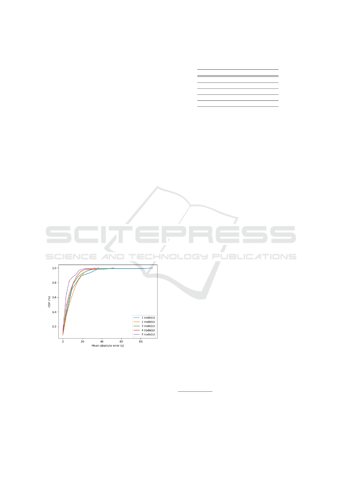
ble. The CDF on Fig. 7 gives the completion time

estimation model accuracy according to the tolerance

(and according to the number of nodes), and Table 3

gives the accuracy corresponding to 15 s according to

the number of cores. This accuracy increases with the

number of nodes, meaning that the simulation reaches

the scale-out property.

Figure 7: CDF according to the mean absolute error be-

tween real completion and prediction. Each chetemi node

has 20 cores. Reachy sends 400 requests to Fog nodes.

5.1.2 Simulation Accuracy Evaluation

Figure 8 gives the evolution of the life-cycle dura-

tion (in real and in simulation) according to the or-

der of the request sent for each conﬁguration of the

Fog layer. This life-cycle consists of three steps (ex-

Table 3: Completion time accuracy for a tolerance of 15 s,

according to the number of nodes.

Number of cores Accuracy (%)

20 80.83

40 80.92

60 88.3

80 90.0

100 96.5

tract, transform and load) and is traced for each re-

quest in simulation and in real deployment to com-

pare both deployments. According to the number of

cores, the difference between both life-cycles dura-

tion in average is short (22.97 s by computing mean

value of CT MAE column of Table 2 giving an accu-

racy of 95% in average for the completion time esti-

mation model) . This tolerance can be considered as

short because it does not really have an impact on the

global makespan, completion time and duration of the

activity, since requests are asynchronous. Despite the

fact that the data communicated by the queries are of

the same order (because standard deviation of image

size distribution (Table 2) is very lower than the mini-

mum value of this distribution (Table 4)), the comple-

tion times in real life vary greatly (Table 2). This is

because at certain times there are many more requests

sharing the CPU than at other times. The simulation

follows this same observation well with respect to the

mean absolute errors of the completion time for each

conﬁguration of the Fog layer highlighted in Table 2.

5.2 Fog Resource Needs Estimation

To implement SERFRI on the use case presented in

Section 2, we consider that Fog instances have simi-

lar characteristics to OVHCloud instances

designed

for data analysis and data-science uses: r2-15, r2-30,

r2-60 , r2-120 and r2-240. We simulate the platform

scenario made-up of : 2, 4, 8, 16, 32 and 64 resources

for each of OVHCloud instance types considered. We

present ﬁrst the simulation settings, then the pareto

optimization and ﬁnally the SERFRI steps: (i) phi-

transformation

, (ii) sigma-transformation

and re-

sult expression.

5.2.1 Settings

To perform the simulations with these new instances,

we do not rebuild an estimation model but we rely on

the models built with the chetemi nodes. Indeed, with

regard to Equation (6)), the workload of a request i

Cloud pricing: Comparison of public Cloud offers-

OVH, https://www.ovhCloud.com/fr/public-Cloud/prices/

The application of φ function

The application of σ function

Simulation-Based Estimation of Resource Needs in Fog Robotics Infrastructures

107

(a) 1 chetemi node: 20 process-

ing cores.

(b) 2 chetemi nodes: 40 pro-

cessing cores.

(d) 4 chetemi nodes: 80 processing

cores.

(e) 5 chetemi nodes: 100 processing

cores.

Figure 8: Requests life-cycle durations. Comparison between Real and Simulation deployments.

on a resource j with speed v

is written W

i j

= t

i j

× v

in the same way, this request processed by another

type of resource of order j with speed v

will have

a workload that will be written W

i j

= t

i j

× v

. This

allows us to deduce the desired completion time: t

i j

×v

Table 4: Simulation settings.

Number of requests 5000

Frequency

(number of

requests/second)

Maximum number

of instances

Bandwidth between

Edge and

Fog Layers (Mbps)

Latency between

Edge and

Fog Layers (s)

0.005

Data sizes range (B) 420000 - 480000

Response json size (B) 62

Instances

(ovh Cloud instances)

r2-15, r2-30,

r2-60, r2-120,

r2-240

Table 4 gives the values of the simulator inputs.

Regarding the characteristics of the instances, the

level of granularity is very low, because we consider:

the memory, the storage, the number of cores, the re-

sources cost per unit of time, the clock frequency, the

maximum number of operations per instruction cycle

and bandwidth in a public network. Requests sizes are

randomly generated between 420000 B and 480000

B, and we keep this same distribution for all deploy-

ment scenarios of the use case.

5.2.2 The Pareto Optimization

Table 5: Makespan (in second) by resource type and con-

ﬁguration.

Conﬁguration R2-15 R2-30 R2-60 R2-120 R2-240

2 82182.11 82182.11 41138.88 20610.64 10253.34

4 41138.88 41138.88 20610.64 10592.45 5591.26

8 20610.64 20610.64 10592.45 5591.26 2690.48

16 10592.45 10592.45 5591.26 2772.42 1530

32 5591.26 5591.26 2772.42 1530 869.8

64 2772.42 2772.42 1530 869.8 494.5

Table 6: Financial cost (in euro) by resource type and con-

ﬁguration.

Conﬁguration R2-15 R2-30 R2-60 R2-120 R2-240

2 4.43 5.12 5.01 5.04 4.95

4 4.45 5.14 4.98 5.09 5.13

8 4.41 5.1 5.01 5.14 5.05

16 4.46 5.15 5.03 5.12 5.22

32 4.45 5.14 5.04 5.28 5.44

64 4.44 5.13 5.16 5.46 6.4

Table 5 and Table 6 present the makespan and

ﬁnancial costs of using Fog resources, respectively.

They are therefore the matrices we referred to in

Section 4.4. The graphical transcription of Table 5

(Fig. 9) shows that the makespan decreases as the

number of resources increases and more so when the

type of resources is more powerful. The graphical

transcription of Table 6 (Fig. 10) , on the other hand,

CLOSER 2023 - 13th International Conference on Cloud Computing and Services Science

108

Figure 9: Makespan by the number of resources for each

type of resource.

Figure 10: Financial cost by the number of resources for

each type of resource.

grows as the number of resources increases and more

so when the type of resources is more powerful, that

makes the optimization very difﬁcult. By naively ap-

plying Pareto optimization to reduce the makespan

and the cost of using resources as much as possible,

we obtain the following Pareto front: {(r2-15, 8), (r2-

15, 64), (r2-60, 64), (r2-240, 8), (r2-240, 32), (r2-240,

64)}.

5.2.3 Phi-Transformation

Table 7 and Table 8 represent the normalized (phi-

transformed tables obtained by applying φ function of

Equation (7)) tables from Table 5 and Table 6 respec-

tively. In other words, we look for the smallest ele-

ment in Table 5 and we calculate for each element of

this table the relative error with respect to this smallest

element, and the same thing is done for the Table 6.

This allows to bring the makespan and the ﬁnancial

cost into the same dimensional space. The makespan

decreases according to the number of resources and

the power of resources, but it is an inverted observa-

tion for the ﬁnancial cost ratio. The Pareto front is the

same front presented in Section 5.2.2.

Table 7: Makespan ratios by resource type and conﬁgura-

tion.

Conﬁguration R2-15 R2-30 R2-60 R2-120 R2-240

2 165.19 165.19 82.19 40.68 19.73

4 82.19 82.19 40.68 20.42 10.31

8 40.68 40.68 20.42 10.31 4.44

16 20.42 20.42 10.31 4.61 2.09

32 10.31 10.31 4.61 2.09 0.76

64 4.61 4.61 2.09 0.76 0

Table 8: Financial cost ratios by resource type and conﬁgu-

ration.

Conﬁguration R2-15 R2-30 R2-60 R2-120 R2-240

2 0 0.16 0.14 0.14 0.12

4 0.01 0.17 0.13 0.15 0.16

8 0 0.16 0.14 0.17 0.15

16 0.01 0.17 0.14 0.16 0.18

32 0.01 0.17 0.14 0.2 0.23

64 0.01 0.16 0.17 0.24 0.45

5.2.4 Sigma-Transformation

This transformation applies the σ function (Equation

8) on normalized matrices. Maximizing these matri-

ces (Table 7 and Table 8) leads to the creation of the

Table 9, according to the Equation (8), from which we

can determine the minimum element and therefore the

solution of the Pareto front that in practice is the most

efﬁcient in terms of time and ﬁnancial cost: (r2-240,

64). It is indeed, because compared to the other Pareto

solutions, it saves much more time than it costs.

Table 9: Maximized ratios by resource type and conﬁgura-

tion.

Conﬁguration R2-15 R2-30 R2-60 R2-120 R2-240

2 165.19 165.19 82.19 40.68 19.73

4 82.19 82.19 40.68 20.42 10.31

8 40.68 40.68 20.42 10.31 4.44

16 20.42 20.42 10.31 4.61 2.09

32 10.31 10.31 4.61 2.09 0.76

64 4.61 4.61 2.09 0.76 0.45

6 CONCLUSION

In this article we address the estimation of Fog re-

source requirements (number of resources, memory,

computing and storage capacity of each resource) of

robotics applications. We then proposed an approach

(SERFRI) for estimating static and homogeneous Fog

resource needs based on the simulation of the deploy-

ment of Fog Robotic infrastructures. This approach

aims at providing the best resource type and the best

number of them, compromising the reduction at best

of the makespan and the one of the ﬁnancial cost of

Simulation-Based Estimation of Resource Needs in Fog Robotics Infrastructures

109

using these Fog resources. We implement the ap-

proach on an existing use case (Reachy) which could

also have industrial vocation. The validation of the

simulator on which the approach is based consisted

mainly on the validation of the machine learning mod-

els used (accurate on average at 95 % with a predic-

tion margin of 23 s for each request, not really im-

pacting the global life-cycle duration of the applica-

tion) to estimate the request completion time. This

approach can therefore, also greatly help industrial

companies (and/or those who base their activities on

the use of robots) to have an approximate idea of the

budget required for the activities of their robots on

Fog resources. This approach also saves the ﬁnan-

cial budget and the use of the robot’s battery, allow-

ing it to perform more tasks. However, a similar ap-

proach should be implemented in the generic case of

platform, where Fog resources are heterogeneous and

dynamic and robots are mobile. The study indeed de-

serves reﬂection because it is not just an implementa-

tion of the knapsack problem as in the case of static

heterogeneous resources.

ACKNOWLEDGEMENTS

We are deeply grateful to all those who played a

role in the success of this project. We would like

to thank Interreg AiBLE and REACT-EU UV-Bot for

their support throughout the research process.

REFERENCES

Aazam, M. and Huh, E.-N. (2015). Fog computing mi-

cro datacenter based dynamic resource estimation and

pricing model for iot. In 2015 IEEE 29th International

Conference on Advanced Information Networking and

Applications, pages 687–694.

Casanova, H., Giersch, A., Legrand, A., Quinson, M.,

and Suter, F. (2014). Versatile, scalable, and accu-

rate simulation of distributed applications and plat-

forms. Journal of Parallel and Distributed Comput-

ing, 74(10):2899–2917.

Chen, Y. and Hu, H. (2013). Internet of intelligent things

and robot as a service. Simulation Modelling Practice

and Theory, 34:159–171.

Deb, K., Pratap, A., Agarwal, S., and Meyarivan, T. (2002).

A fast and elitist multiobjective genetic algorithm:

Nsga-ii. IEEE transactions on evolutionary compu-

tation, 6(2):182–197.

Garcia, J., Sim

o, E., Masip-Bruin, X., Mar

ı-Tordera, E., and

anchez-L

opez, S. (2018). Do we really need cloud?

estimating the fog computing capacities in the city of

barcelona. In 2018 IEEE/ACM International Con-

ference on Utility and Cloud Computing Companion

(UCC Companion), pages 290–295.

Gudi, S. C. et al. (2017). Fog robotics: An introduction.

In IEEE/RSJ International Conference on Intelligent

Robots and Systems.

Gupta, H., Vahid Dastjerdi, A., Ghosh, S. K., and Buyya,

R. (2017). ifogsim: A toolkit for modeling and

simulation of resource management techniques in

the internet of things, edge and fog computing en-

vironments. Software: Practice and Experience,

47(9):1275–1296.

Johnson, S. G. (2014). The nlopt nonlinear-optimization

package.

Kapitonov, A., Lonshakov, S., Bulatov, V., Kia, B., and

White, J. (2021). Robot-as-a-service: From cloud

to peering technologies. In 2021 The 4th Interna-

tional Conference on Information Science and Sys-

tems, pages 126–131.

Kattepur, A., Rath, H. K., and Simha, A. (2017). A-priori

estimation of computation times in fog networked

robotics. In 2017 IEEE international conference on

edge computing (EDGE), pages 9–16. IEEE.

Koubaa, A. (2014). A service-oriented architecture for vir-

tualizing robots in robot-as-a-service clouds. In In-

ternational Conference on Architecture of Computing

Systems, pages 196–208. Springer.

Kunde, C. and Mann, Z.

A. (2020). Comparison of simu-

lators for fog computing. In Proceedings of the 35th

annual ACM symposium on applied computing, pages

1792–1795.

Kwon, M., Biyik, E., Talati, A., Bhasin, K., Losey, D. P.,

and Sadigh, D. (2020). When humans aren’t opti-

mal: Robots that collaborate with risk-aware humans.

In 2020 15th ACM/IEEE International Conference on

Human-Robot Interaction (HRI), pages 43–52. IEEE.

Lera, I., Guerrero, C., and Juiz, C. (2019). Yafs: A simula-

tor for iot scenarios in fog computing. IEEE Access,

7:91745–91758.

Lopes, M. M., Higashino, W. A., Capretz, M. A., and Bit-

tencourt, L. F. (2017). Myifogsim: A simulator for

virtual machine migration in fog computing. In Com-

panion Proceedings of the10th International Confer-

ence on Utility and Cloud Computing, pages 47–52.

Mick, S., Lapeyre, M., Rouanet, P., Halgand, C., Benois-

Pineau, J., Paclet, F., Cattaert, D., Oudeyer, P.-Y., and

De Rugy, A. (2019). Reachy, a 3d-printed human-

like robotic arm as a testbed for human-robot control

strategies. Frontiers in neurorobotics, 13:65.

Moniz, A. B. and Krings, B.-J. (2016). Robots working with

humans or humans working with robots? searching

for social dimensions in new human-robot interaction

in industry. Societies, 6(3):23.

Mushunuri, V., Kattepur, A., Rath, H. K., and Simha, A.

(2017). Resource optimization in fog enabled iot de-

ployments. In 2017 Second International Conference

on Fog and Mobile Edge Computing (FMEC), pages

6–13. IEEE.

Ngatchou, P., Zarei, A., and El-Sharkawi, A. (2005). Pareto

multi objective optimization. In Proceedings of the

CLOSER 2023 - 13th International Conference on Cloud Computing and Services Science

110

13th international conference on, intelligent systems

application to power systems, pages 84–91. IEEE.

Norman, D. A. and Bobrow, D. G. (1975). On data-limited

and resource-limited processes. Cognitive psychology,

7(1):44–64.

Papazoglou, M. P. and Van Den Heuvel, W.-J. (2007). Ser-

vice oriented architectures: approaches, technologies

and research issues. The VLDB journal, 16(3):389–

415.

Quigley, M., Conley, K., Gerkey, B., Faust, J., Foote, T.,

Leibs, J., Wheeler, R., Ng, A. Y., et al. (2009). Ros: an

open-source robot operating system. In ICRA work-

shop on open source software, volume 3, page 5.

Kobe, Japan.

R. de Oliveira., E., Delicato., F., R. da Rocha., A., and

Mattoso., M. (2021). A real-time and energy-aware

framework for data stream processing in the internet

of things. In Proceedings of the 6th International Con-

ference on Internet of Things, Big Data and Security -

IoTBDS,, pages 17–28. INSTICC, SciTePress.

Ray, P. P. (2016). Internet of robotic things: Concept, tech-

nologies, and challenges. IEEE access, 4:9489–9500.

Sakovich, N. (2020). Fog computing vs. cloud computing

for iot projects.

Turnbull, L. and Samanta, B. (2013). Cloud robotics: For-

mation control of a multi robot system utilizing cloud

infrastructure. In 2013 Proceedings of IEEE South-

eastcon, pages 1–4. IEEE.

Velho, P. and Legrand, A. (2010). Accuracy study and

improvement of network simulation in the simgrid

framework. In 2nd International ICST Conference on

Simulation Tools and Techniques.

Zhao, W., Peng, Y., Xie, F., and Dai, Z. (2012). Model-

ing and simulation of cloud computing: A review. In

2012 IEEE Asia Paciﬁc Cloud Computing Congress

(APCloudCC), pages 20–24.

Simulation-Based Estimation of Resource Needs in Fog Robotics Infrastructures

111