Data-Driven Modelling of Freshwater Ecosystems: A Multiscale

Framework Based on Global Geospatial Data

Bruna Almeida

and Pedro Cabral

Information Management School (NOVA IMS), Universidade Nova de Lisboa,

Campus de Campolide, 1070-312 Lisbon, Portugal

Keywords: Remote Sensing, Ecosystem Services, Water Modelling, Machine Learning, Geographical Information

Systems.

Abstract: Freshwater ecosystems are primarily impacted by climate, land use and land cover changes, and over-

abstraction. Satellite Earth observation (SEO) data and technologies are key in environmental modelling and

support decisions. These technologies combined with machine learning (ML) are a powerful approach for

modelling freshwater ecosystems at a multiscale level. The goal of this study is to present a set of reference

data and guidelines that can be used to estimate the water and wetness probability index (WWPI) in different

spatial and temporal scales. To find the best model’s predictors, sensitivity analyses were carried out in a

predictive ML model implemented in a transnational river basin district (Portugal – Spain), the Tagus Basin.

Satellite imagery, satellite-derived data, biophysical variables, and landscape characteristics were the

explanatory variables evaluated in the sensitivity analyses, and some of them were included in the framework

as a reference source of spatial data.

1 INTRODUCTION

Anthropogenic and environmental changes threaten

the existence of ecosystems that depend directly or

indirectly on the presence of water in a landscape

(Mpakairi et al., 2022). Those ecosystems are

biodiversity hotspots that require access to water to

maintain the communities of plants and animals, the

ecological processes they support, and the services

they provide (Shi et al., 2014). In dry periods, there is

less water in rivers, and over-exploitation depletes the

natural water table and affects these vulnerable

ecosystems (Sharma et al., 2018).

The status of water resources degradation and

scarcity gets worse as human activities directly cause

an increase in the local drying initiated by climate

(Kløve et al., 2014). Adverse atmospheric conditions

impact water resource availability, compounding the

challenge of integrated water management,

concerning quality, quantity, and ecosystem support

(Novo et al., 2018). In face of climate change and

ever-more intensive land use, conceptual models, and

quantitative assessments of surface and groundwater

https://orcid.org/0000-0002-3349-1470

https://orcid.org/0000-0001-8622-6008

interactions with the environment are needed (Yang

et al., 2021).

The increasing global demand for water for

agriculture, domestic, and industrial needs, requires

integrated management of natural resources (Almeida

& Cabral, 2021). Therefore, there is a lack of

knowledge on the existence of conceptual

frameworks and guidelines useful to model

freshwater ecosystems (Cui et al., 2021). The process

of acquiring geospatial data is the most challenging

part of environmental modelling (Meddens et al.,

2022). Frameworks to support data-driven modelling

must incorporate the knowledge that facilitates spatial

and spatiotemporal data acquisition and baselines that

guide conceptualization and model implementation

(Nti et al., 2022).

When there are few or no guidelines for sources

of spatial data and environmental applications,

searching and applying exhaustively all the

possibilities is not a feasible option because, even

with very sophisticated computers, the running time

needed would be unacceptable, or could not add any

value for the model in terms of quality. Several

104

Almeida, B. and Cabral, P.

Data-Driven Modelling of Freshwater Ecosystems: A Multiscale Framework Based on Global Geospatial Data.

DOI: 10.5220/0012037800003473

In Proceedings of the 9th International Conference on Geographical Information Systems Theory, Applications and Management (GISTAM 2023), pages 104-111

ISBN: 978-989-758-649-1; ISSN: 2184-500X

 2023 by SCITEPRESS – Science and Technology Publications, Lda. Under CC license (CC BY-NC-ND 4.0)

studies have been developing methodologies for

modelling water ecosystems using remote sensing

and machine learning, such as Kundu et al. (2022)

detecting water richness change, Mpakairi et al.

(2022) assessing spatiotemporal variation of

vegetation heterogeneity in groundwater-dependent

ecosystems, and Sharma et al. (2018) estimating

impacts on the water resources from crop irrigation.

In synthesis, we observe that some of the previously

proposed approaches solve the problem very well, but

none of them was presenting possible sources of

global spatial data and performed a sensibility

analysis of their use and applications in modelling

water ecosystems.

The Copernicus Land Monitoring Services

(CLMS) provides the basis for integrated analysis of

the main drivers of land use change to inform about

Europe’s natural resources and their status

(Copernicus Programme, 2023). It offers information

services based on satellite Earth observation freely

and openly accessible to its users, only requiring

registration and referencing. In the portfolio of the

High-Resolution Layers (HRL) under the Experts and

National Products archive, exist five thematic layers

on land cover characteristics at 10m spatial

resolution, covering 39 European countries. The HRL

Water and Wetness (WAW) 2018 datasets are based

on imagery covering the period 2012-2018. They

were created based on satellite imagery, including

ESA’s Sentinel-1 and Sentinel-2 satellites and

spectral indices such as the Normalised Difference

Water Index (NDWI) and its modified version

mNDWI, as well as the Normalised Difference

Vegetation Index (NDVI).

The goal of this study is to present a set of

reference data and application guidelines that support

reproducing the WWPI with accuracy. For that, we

developed machine learning (ML) models and

performed sensitivity analyses to find the best

predictors. The ML models were implemented in a

transnational river basin district (Portugal – Spain),

the Tagus Basin. Satellite imagery, satellite-derived

data, biophysical variables, and landscape

characteristics were the explanatory variables

evaluated in the sensitivity analyses.

The framework comprises a set of global open-

access data, that can be used to model freshwater

ecosystems at multiscale (spatial and spatiotemporal).

The outcomes of this research would increase our

understanding of the use and replicability of the

Copernicus data, and knowledge in implementing

data-driven models based on SEO data in different

years and locations. The developed framework

comprises a set of baselines for predicting the spatial

distribution of water and wetness status and

conditions allowing the assessment of the impacts of

drivers of changes on freshwater ecosystems.

2 MATERIALS & METHODS

2.1 Study Area

The Tagus Basin in Portugal is the most important

source of water in the country due to its productivity,

and quality of water (Ribeiro, 1998). The river basin

resources are responsible for economic and

demographic expansion through the years

(Mendonça, 1990).

The extensive network drainage promotes easy

access to water and supports the development of

intensive agriculture (Almeida, 2020), such as

annually harvested plants including flooded crops

such as rice fields and other inundated croplands, and

permanent crops such as vineyards, fruit trees and

olive groves (Novo et al., 2018). Forest and

seminatural areas are represented by mixed forest and

transitional woodland/shrub (Ramos et al., 2017).

Due to its strategic location in the surroundings of

Lisbon, the most populated region of the country,

there is a growing need for changes in land use to

develop artificial surfaces such as urban fabric, road

and rail networks, airports, dump sites and industrial

areas (Mendes et al., 2015), which is compromising

water resources and dependent ecosystems in the

basin.

2.2 Data Source

2.2.1 Dependent Variable

The necessary data to implement a learning machine

process is commonly divided into training, validation,

and test datasets (Domingos, 2012). The training data

are the predictors, the validation dataset is used to

control the learning process and the test dataset is

employed to assess the learner's performance. To

predict continuous values such as the Water and

Wetness Probability Index (WWPI), regression tasks

were carried out. The target in the regression models

is the response variable, also known as dependent

variable.

The WWPI is a raster displaying the occurrence

of water and wet areas as an index on a scale between

0 (only dry observations) to 100 (only water

observations) (Copernicus Programme, 2023). It

indicates the degree of wetness in a physical sense,

independently of the actual vegetation cover. The

Data-Driven Modelling of Freshwater Ecosystems: A Multiscale Framework Based on Global Geospatial Data

105

landscape elements included in the datasets are

permanent and temporary open water bodies,

temporarily inundated areas, wet agricultural fields,

and transitional coastal water bodies (European

Environment Agency, 2023).

2.2.2 Explanatory Variables

The main goal of this study is to find the best

predictors to enable an accurate reproducibility of the

WWPI dataset. A wide variety of data such as satellite

imagery, satellite-derived data, biophysical variables,

and landscape characteristics, were evaluated through

sensitivity analysis.

Single bands from Sentinel-2 images and satellite-

derived indices were the first predictors evaluated in

the sensitivity analysis. This satellite has a high-

resolution multispectral sensor acquiring and

recording information in 13 bands: visible (VIS with

4 bands), near-infrared (NIR with 6 bands) and

shortwave infrared (SWIR with 3 bands). This

instrument can detect small differences in spectral

signatures, as they have contiguous bands with small

bandwidths (<20 nm), and consequently acquire more

accurate information (Hunter et al., 2020). The

Sentinel-2 mission is providing data from 2015 until

2025 with a temporal resolution of 5 days, and spatial

resolution of 10, 20 and 60m.

The combination of algebraic operations in pre-

established bands leads to the definition of indices

that allow highlighting certain information (i.e.,

water, vegetation, soil, minerals, etc.). Spectral-

derived indices result from combinations of two or

more spectral bands designed for the enhancement of

specific objects (Kuenzer et al., 2014). NDVI, NDWI

and Normalized Difference Moisture Index (NDMI)

were calculated and included as predictors.

Climate variables, such as precipitation and

evapotranspiration combined with topography are

important drivers in water modelling (Ringersma et

al., 2003). The annual precipitation was obtained

from the WorldClim database (Fick & Hijmans,

2017) and the Global Potential Evapotranspiration

(Global-PET) and the Global Aridity Index (Global-

Aridity) from the Consortium of Spatial Information,

Global-Aridity and Global-PET Database (Trabucco

& Zomer, 2019). Global data precipitation was

obtained from spatial interpolation of nearly 60 000

weather stations providing monthly climate data. The

datasets have a spatial resolution of approximately

1 km

. Reference evapotranspiration and global

aridity were derived from the WorldClim

precipitation model and have the same spatial

resolution and temporal scale.

Topographic data are globally available from

NASA through the Shuttle Radar Topography

Mission (SRTM). The dataset was released in the year

2000 with approximately 30m pixel resolution.

Table 1 lists the datasets used to estimate WWPI,

specifying the source of data and the pixel resolution.

Table 1: Description of the datasets, its source and pixel

resolution.

Data Source Pixel

resolution

Satellite Data Copernicus Open Access

Hub

(https://scihub.copernicus.

eu/)

10m

Digital Elevation

Model (DEM)

NASA Shuttle Radar

Topography Mission

(https://www.earthdata.na

sa.gov/)

30m

Average Annual

Precipitation

(mm)

WorldClim

(https://worldclim.org/)

1km

Global Potential

Evapotranspiration

(Global-PET) (mm)

Consortium of Spatial

Information-CSI

(http://www.cgia

-csi.org)

1km

Global Aridity

Index (Global-

Aridity)

Consortium of Spatial

Information-CSI

(http://www.cgia

-csi.org)

1km

2.3 Model Design

In regression problems, the target values are

continuous, and the machine consistently improves

learning to better fit the model. The expected output

was a predictive spatial model implemented in a

geographic information system using ArcGIS Pro

2.9.0 software (ESRI, 2022). The task was to build a

regression model using a non-parametric approach

that enables the replicability of the WWPI with

accuracy. The relationship between explanatory

variables and the response variable was modelled

through the tool Train Random Trees Regression

Model.

The Random Trees algorithm is an adaptation of

the Decision trees (DT) (Breiman, 1984) in a GIS

environment. It is a nonparametric approach that

iteratively divides a dataset into increasingly smaller

subgroups using the same splitting decision (Zhang et

al., 2019). The decisions are made according to the

rank order of importance, optimized by a randomized

procedure (Mallinis et al., 2020). DT can inherently

handle nonlinear relationships, mixed predictor

categories, and data gaps, and are resistant to outliers

and the effects of collinearity (Osborne & Alvares-

Sanches, 2019). The disadvantage of the DT is related

to the models’ fitness and instability due to the

GISTAM 2023 - 9th International Conference on Geographical Information Systems Theory, Applications and Management

106

propagation of errors down through subsequent splits

in the tree (Breiman, 2001).

The input datasets comprising the explanatory

variables and the target were in raster data format. As

the cell size affects the training result and the

processing time, this parameter was set up in the

environment settings to make sure that the training

process will keep the pixel size of 10m, as same as the

target. The Percent Samples for Testing was set to

20%, meaning that one-fifth of the training sample

was used to measure the error for interpolation in

space, called test location points. This parameter

evaluates three types of errors: errors on training

points, errors on test points, and errors on test location

points. The maximum number of trees, the maximum

tree depth and the maximum number of samples were

set by default with values of 50, 30 and 100000,

respectively. The maximum depth of each tree refers

to the number of rules each tree is allowed to create

to come to a decision.

Evaluating regression performance is crucial to

understand how well the model is fitted and explained

by independent variables. Coefficient of

determination (R-squared) and regression error (Re)

were the metrics used to detect bias and the

proportion of variance of the response variable. A

table containing information describing the

importance of each predictor used in the model was

provided as output by the tool, as well as scatterplots

of training data, test data, and test location data, and

the regression definition file contains attribute

information, statistics, and model performance.

2.4 Sensitivity Analysis

Sensitivity analyses were carried out following the

process shown in Figure 1.

The diagram flow has three main steps: modelling the

relationship between the response variable and

predictors, measuring the model’s performance, and

optimizing the model. To build the best framework a

set of global environmental variables were modelled,

the goodness of fit was checked, and the model was

optimized as needed. This process was applied twice,

on a satellite image sensed on 25/04/2018 and another

on 18/08/2018.

Table 1: Description of the explanatory variables included

in each model test.

Model Ex

lorator

variable

M1 Satellite data (Single

ands)

M2 Satellite-derive

data (NDVI, NDWI, NDMI)

M3 M1 + M2

M4 M3 + Di

ital Elevation Model

(

)

M5 M4 +Avera

e annual

reci

itation

(

)

M6 M5 + Average annual potential

evapotranspiration (mm)

M7 M6 + Annual aridit

index

2.5 Models Deployment

The most skilled model resulting from the sensitivity

analysis was deployed in two different scenarios. One

was applying the framework to model landscape

water resources on a Sentinel-2 image sensed on

Figure 1: Diagram flow of sensitivity analysis.

Data-Driven Modelling of Freshwater Ecosystems: A Multiscale Framework Based on Global Geospatial Data

107

29/01/2022, called temporal deployment. The second

deployment was on an image taken on 23/08/2018 in

another area (decimal geographic bounding box -

Longitude: west = 350.99 and east = 352.28; and

Latitude: south = 38.75 and north = 39.75), what was

called a spatial deployment. Satellite-derived indices

were calculated for both images to apply the

framework.

3 RESULTS

3.1 Sensitivity Analysis

The outputs of the training process were analysed to

measure the goodness of predictions. The tool checks

for three types of errors: errors on training points,

errors on test points, and errors on test location points.

Table 3 shows the models’ performance with values

for the regression error (Re) at train locations (80% of

all locations) and test locations (20% of all locations),

and R-squared for training data, test data and test

locations. The models are grouped by image date

sensed, where sp refers to the image taken on

25/04/2018 and sm on 18/08/2018.

Table 3: Models performance grouped by image date

sensed. Legend: TrTr (training data at training locations),

TeTr (test data at training locations), and TeTe (test data at

test locations), Re (regression error).

TrT

TeT

TeTe

Model Re R

Re R

M1_sp 1.289 0.960 2.904 0.872 3.913 0.894

1.827 0.924 3.751 0.777 5.258 0.809

M3_sp 1.278 0.960 2.925 0.871 3.908 0.892

1.004 0.957 2.490 0.820 3.413 0.851

M5_sp 0.901 0.961 2.134 0.841 3.001 0.850

0.801 0.962 1.980 0.800 2.706 0.811

M7_sp 0.801 0.966 1.980 0.820 2.827 0.825

1.218 0.954 2.488 0.848 3.541 0.878

M2_s

1.675 0.909 3.189 0.739 4.491 0.779

1.191 0.951 2.455 0.835 3.431 0.886

0.887 0.953 2.220 0.785 3.108 0.772

0.771 0.958 1.950 0.805 2.652 0.824

0.725 0.962 1.816 0.814 2.571 0.829

0.722 0.962 1.830 0.789 2.490 0.839

The best performance was in model M7 for both

dates. Models’ predictors were the single bands,

spectral indices, topography, precipitation, potential

evapotranspiration, and aridity index. The image

sensed on 18/08/18 has better results regarding Re

than the first image.

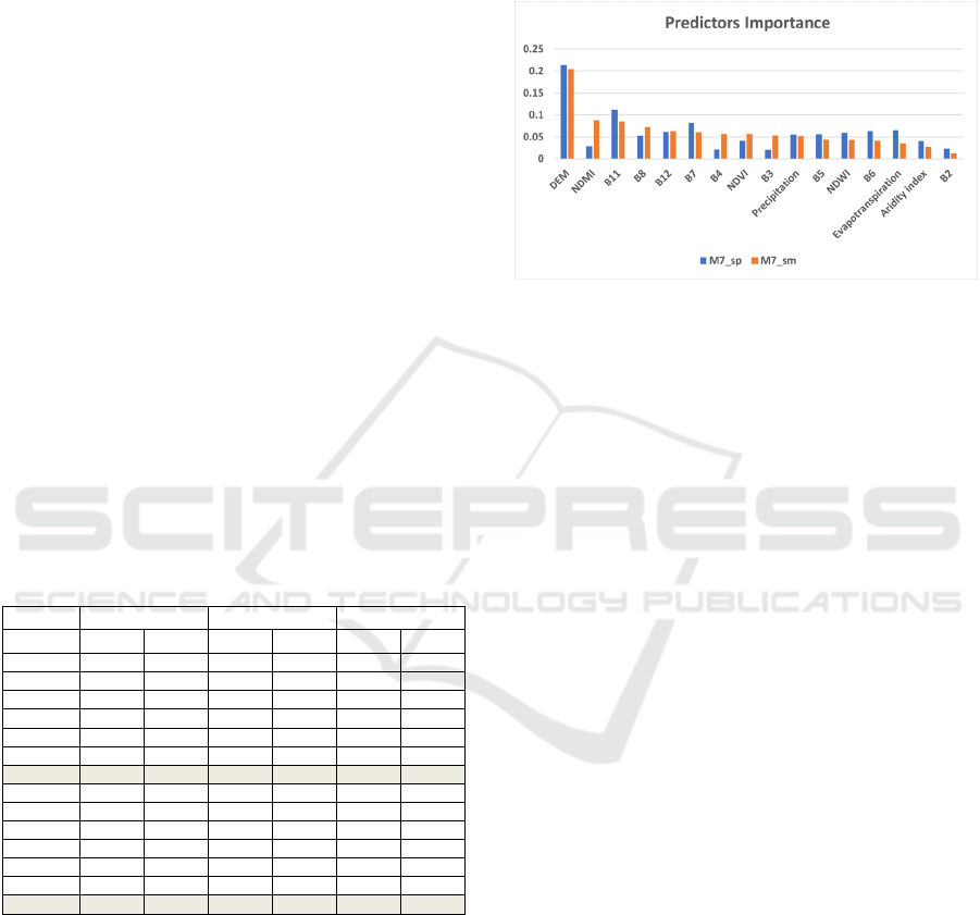
Figure 2 is describing the importance of each

predictor used in the models. The variables with the

highest values are more correlated to the target and

more relevant to the model. Values range between 0

and 1, and the sum of all the values equals 1.

Topography was the predictor that most

contribute to both models (M7_sp and M7_sm). The

predictors’ importance varies widely between

models. All variables showed to be important for the

models, except for the single band B2 in the model

M7_sm, and B3, B4 and NDMI for M7_sp.

Figure 2: Predictors’ importance for the best model in each

group of sensitivity analysis tests.

3.2 Models Deployment

The framework was deployed to evaluate the

temporal and spatial goodness of fit of the selected

model. The ML regression tool measured R-squared

and regression errors (Re) as the main evaluation

measures of the goodness of predictions. The

comparison of the true values with predicted values

was done in terms of errors (standard error of the

regression), the proportion of variance (R-squared)

and plotting the residuals over targets. The first

deployment was applying the framework at the study

area but on another date (29/01/2022).

Figure 3 displays a scatterplot of predictions over-

reference values and the residual plot. The R-squared

is comparable with those obtained in the sensitivity

analysis, with results showing very closed values, and

the residual plot presenting few outliers, especially on

the test data at test locations and training locations.

Meaning that in locations where the WWPI detected

no water (WWPI equals zero), the model predicted

some degree of wetness. This can be explained by

analysing the sensed date, which is from a

Mediterranean wet season (29/01/2022), and on that

day these locations could be flooded, or the soil

moisture was higher than it used to be in the spring

and summer.

The framework performance was also evaluated

by deploying it using a satellite image from another

area. Figure 4 shows the scatterplot of predictions

over observed values and the residual plot of the

spatial deployment.

GISTAM 2023 - 9th International Conference on Geographical Information Systems Theory, Applications and Management

108

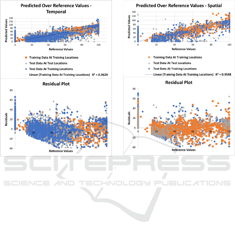
Figure 3: Scatterplot and residual plot of the temporal

deployment applying the framework.

Comparing both deployments, the R-squared was

better at applying the framework in the same study

area rather than applying it to the other region. We

also analysed R-squared and Re for test data at

training locations and test data at test locations, and

the overall results were better in the study area. The

residuals are presenting some outliers, but more

sparsely than the residual plot of the first deployment.

4 DISCUSSIONS

Water diversion and livestock grazing are threatening

the functionality of many natural systems, which

increases the impacts that a warmer climate may

bring. When inland wetlands, rivers, and lakes, gets

fragmented and become hydrologically inconsistent,

the values they produce change, and can rapidly

decrease. Assessing water resources at an appropriate

management scale is a necessary step for the

sustainable management of natural resources.

The HRL developed by CLMS are designed for

use by a broad user community as the basis for

environmental and regional analyses and for

Figure 4: Spatial deployment at the study area applying the

framework.

supporting political decision-making (European

Environment Agency, 2023). They include

geographical information on land cover and its

changes, land use, vegetation state, water cycle and

earth surface energy variables freely available at the

European scale.

They were built based on high-resolution satellite

data globally available. High spatial resolution

sensors represent a smaller area of land, but with

more detail and accuracy (Liang & Wang, 2019).

However, higher resolution implies larger files, more

loading, viewing, and processing time and more space

taken up in databases, which can be a limitation. But

also building environmental monitoring systems

based on ML models require powerful computational

resources, and most of the time a large amount of

data.

ML models are only as accurate as the data they

are fed in. The most known law of modelling saying,

“garbage in, garbage out”, could be shown here if we

did not carefully select the data to be included in the

framework. Large margins of error in the predictors

prevent the model from being considered correct.

Models with lower error and higher R-squared are

indications of higher skill predictions. Nevertheless,

Data-Driven Modelling of Freshwater Ecosystems: A Multiscale Framework Based on Global Geospatial Data

109

none of those functions alone is enough to validate a

model’s predictions. Using a combination of

evaluation metrics is recommended, to assess the

differences between observed data and predictions, to

compare models’ performance, and quantify the

explained variance.

Water yield and soil moisture content are some

examples of ecosystem functions that are highly

dependent on climatic and topographic drivers such

as precipitation, evapotranspiration, temperature, and

elevation. Topographic variables such as elevation

and slope are very important drivers in ecological

models. The topography creates specific habitats and

influences the occurrence of certain plant species, as

in wetlands, an ecosystem that predominantly occurs

in flat landscapes, with a very low slope degree. The

results show that elevation was the most important

feature in both images tested, followed by the single

band B11 (SWIR). The shortwave infrared bands

highlight water content in vegetation.

The developed framework requires more

deployment tests in different locations and time

frames. Future work will expand the methodology to

assess the relationship between ecosystem services

and water resources at the national scale flagging the

location and characteristics of water-dependent

ecosystems across Portugal. But also, further research

is needed to evaluate other ML algorithms and

explore other spectral indices and landscape metrics

that can be included as reference data in the

framework. As well as testing other SEO data such as

from the GRACE (Gravity Recovery and Climate

Experiment) satellite mission that is used to identify

regional trends of freshwater movement on the earth’s

surface and compare results.

5 CONCLUSIONS

The framework support studies related to the spatial

estimation of water availability at the European level

with the possibility of being implemented multiscale,

as it includes global open-access data. The time

capability of predictions depends on the launch date

of the satellite data used. The comparison of models

was important to build confidence in the selected

predictors.

The outcomes of this study guide future research

to make better use of the globally available data that

can be used as predictors in data-driven water

modelling. Also, to advance the knowledge of the

datasets provided by CLSM at the European level.

The developed framework requires more deployment

tests, nevertheless, model deployment had shown

overall good results, and the capability of being used

worldwide as a baseline for modelling freshwater

ecosystems.

ACKNOWLEDGEMENTS

This work was supported by the research project

MaSOT – Mapping Ecosystem Services from Earth

Observations, funded by the Portuguese Science

Foundation – FCT [EXPL/CTA-AMB/0165/2021],

and by national funds through FCT (Fundação para a

Ciência e a Tecnologia), under the project -

UIDB/04152/2020 - Centro de Investigação em

Gestão de Informação (MagIC)/NOVA IMS.

REFERENCES

Almeida, B. (2020). Estudo Hidrogeológico no Sistema

Aquífero Aluviões do Tejo: contributo para a

sustentabilidade da massa de água subterrânea.

http://hdl.handle.net/10451/45261

Almeida, B., & Cabral, P. (2021). Water yield modelling,

sensitivity analysis and validation: A study for

Portugal. ISPRS International Journal of Geo-

Information, 10(8). https://doi.org/10.3390/ijgi10080

494

Breiman, L. (1984). Classification and regression trees (1st

ed.). Routledge. https://doi.org/10.1201/97813151394

Breiman, L. (2001). Random forests. Machine Learning,

45(1), 5–32. https://doi.org/10.1023/A:1010933404324

Copernicus Programme. (2023). CLC 2018 — Copernicus

Land Monitoring Service. https://land.copernicus.eu/

pan-european/corine-land-cover/clc2018

Cui, Q., Ammar, M. E., Iravani, M., Kariyeva, J., &

Faramarzi, M. (2021). Regional wetland water storage

changes: The influence of future climate on

geographically isolated wetlands. Ecological

Indicators, 120. https://doi.org/10.1016/j.ecolind.20

20.106941

Domingos, P. (2012). A few useful things to know about

machine learning. In Communications of the ACM (Vol.

55, Issue 10, pp. 78–87). https://doi.org/10.1145/

2347736.2347755

ESRI. (2022). ArcGIS - ESRI (Environmental Systems

Research Institute). https://www.arcgis.com/index.

html

European Environment Agency. (2023). Copernicus Land

Monitoring Service.

Fick, S. E., & Hijmans, R. J. (2017). WorldClim 2: new 1-

km spatial resolution climate surfaces for global land

areas. International Journal of Climatology, 37(12),

4302–4315. https://doi.org/https://doi.org/10.1002/joc.

5086

GISTAM 2023 - 9th International Conference on Geographical Information Systems Theory, Applications and Management

110

Hunter, F. D. L., Mitchard, E. T. A., Tyrrell, P., & Russell,

S. (2020). Inter-seasonal time series imagery enhances

classification accuracy of grazing resource and land

degradation maps in a savanna ecosystem. Remote

Sensing, 12(1), 198. https://doi.org/10.3390/RS12010

198

Kløve, B., Ala-Aho, P., Bertrand, G., Gurdak, J. J.,

Kupfersberger, H., Kværner, J., Muotka, T., Mykrä, H.,

Preda, E., Rossi, P., Uvo, C. B., Velasco, E., & Pulido-

Velazquez, M. (2014). Climate change impacts on

groundwater and dependent ecosystems. Journal of

Hydrology, 518(PB), 250–266. https://doi.org/10.1016/

J.JHYDROL.2013.06.037

Kuenzer, C., Ottinger, M., Wegmann, M., Guo, H., Wang,

C., Zhang, J., Dech, S., & Wikelski, M. (2014). Earth

observation satellite sensors for biodiversity

monitoring: potentials and bottlenecks. In International

Journal of Remote Sensing (Vol. 35, Issue 18, pp.

6599–6647). Taylor and Francis Ltd. https://doi.org/

10.1080/01431161.2014.964349

Kundu, S., Pal, S., Mandal, I., & Talukdar, S. (2022). How

far damming induced wetland fragmentation and water

richness change affect wetland ecosystem services?

Remote Sensing Applications: Society and

Environment, 27, 100777. https://doi.org/10.1016/

j.rsase.2022.100777

Liang, S., & Wang, J. (2019). Advanced remote sensing:

Terrestrial information extraction and applications.

Advanced Remote Sensing: Terrestrial Information

Extraction and Applications, 1–986. https://doi.org/

10.1016/C2017-0-03489-4

Mallinis, G., Chrysafis, I., Korakis, G., Pana, E., &

Kyriazopoulos, A. P. (2020). A random forest

modelling procedure for a multi-sensor assessment of

tree species diversity. Remote Sensing, 12(7), 1210.

https://doi.org/10.3390/rs12071210

Meddens, A. J. H., Steen-Adams, M. M., Hudak, A. T.,

Mauro, F., Byassee, P. M., & Strunk, J. (2022).

Specifying geospatial data product characteristics for

forest and fuel management applications.

Environmental Research Letters, 17(4). https://doi.org/

10.1088/1748-9326/ac5ee0

Mendes, M. P., Paralta, E., Batista, S., & Cerejeira, M. J.

(2015). Vulnerabilidade, monitorização e risco na zona

vulnerável do Tejo. 8

Congresso Da Água.

Mendonça, J. J. L. (1990). Estudo Estatístico dos

Parâmetros Hidráulicos do Sistema Aquífero Aluvionar

do Tejo.

Mpakairi, K. S., Dube, T., Dondofema, F., & Dalu, T.

(2022). Spatio–temporal variation of vegetation

heterogeneity in groundwater dependent ecosystems

within arid environments. Ecological Informatics, 69,

101667. https://doi.org/10.1016/j.ecoinf.2022.101667

Novo, M. E., Oliveira, M., Martins, T., & Henriques, M. J.

(2018). Projecto Bingo: O Impacto das Alterações

Climáticas na Componente Subterrânea do Ciclo

Hidrológico. Revista Recursos Hídricos, 39(2), 59–74.

https://doi.org/10.5894/rh39n2-cti3

Nti, E. K., Cobbina, S. J., Attafuah, E. E., Opoku, E., &

Gyan, M. A. (2022). Environmental sustainability

technologies in biodiversity, energy, transportation and

water management using artificial intelligence: A

systematic review. Sustainable Futures, 4, 100068.

https://doi.org/10.1016/J.SFTR.2022.100068

Osborne, P. E., & Alvares-Sanches, T. (2019). Quantifying

how landscape composition and configuration affect

urban land surface temperatures using machine learning

and neutral landscapes. Computers, Environment and

Urban Systems, 76, 80–90. https://doi.org/10.1016/

j.compenvurbsys.2019.04.003

Ramos, T. B., Horta, A., Gonçalves, M. C., Pires, F. P.,

Duffy, D., & Martins, J. C. (2017). The INFOSOLO

database as a first step towards the development of a

soil information system in Portugal. Catena, 158(July),

390–412. https://doi.org/10.1016/j.catena.2017.07.020

Ribeiro, M. M. S. (1998). Contribuição para o

conhecimento hidrogeológico do Cenozóico na Bacia

do Baixo Tejo.

Ringersma, J., Batjes, N., & Dent, D. (2003). Green Water:

definitions and data for assessment. ISRIC – World Soil

Information, December, 83.

Sharma, A., Hubert-Moy, L., Buvaneshwari, S., Sekhar,

M., Ruiz, L., Bandyopadhyay, S., & Corgne, S. (2018).

Irrigation History Estimation Using Multitemporal

Landsat Satellite Images: Application to an Intensive

Groundwater Irrigated Agricultural Watershed in India.

Remote Sensing, 10(6), 893. https://doi.org/10.3390/

rs10060893

Shi, H., Li, L., Eamus, D., Cleverly, J., Huete, A., Beringer,

J., Yu, Q., Van Gorsel, E., & Hutley, L. (2014). Intrinsic

climate dependency of ecosystem light and water-use-

efficiencies across Australian biomes. Environmental

Research Letters, 9(10). https://doi.org/10.1088/1748-

9326/9/10/104002

Trabucco, A., & Zomer, R. (2019). Global Aridity Index

and Potential Evapotranspiration (ET0) Climate

Database v2. https://doi.org/10.6084/m9.figshare.750

4448.v3

Yang, X., Liu, S., Jia, C., Liu, Y., & Yu, C. (2021).

Vulnerability assessment and management planning for

the ecological environment in urban wetlands. Journal

of Environmental Management, 298, 113540.

https://doi.org/10.1016/j.jenvman.2021.113540

Zhang, J., Okin, G. S., & Zhou, B. (2019). Assimilating

optical satellite remote sensing images and field data to

predict surface indicators

in the Western U.S.:

Assessing error in satellite predictions based on

large geographical datasets with the use of

machine learning. Remote Sensing of Environment,

233, 111382. https://doi.org/10.1016/j.rse.2019.111382

Data-Driven Modelling of Freshwater Ecosystems: A Multiscale Framework Based on Global Geospatial Data

111