Lessons Learned: Defending Against Property Inference Attacks

Joshua Stock

1 a

, Jens Wettlaufer

, Daniel Demmler

1 b

and Hannes Federrath

Security in Distributed Systems, Universit

at Hamburg, Germany

Institute of Electrical and Electronics Engineers (IEEE), U.S.A.

Keywords:

Machine Learning, Privacy Attacks, Property Inference, Defense Mechanisms, Adversarial Training.

Abstract:

This work investigates and evaluates defense strategies against property inference attacks (PIAs), a privacy

attack against machine learning models. While for other privacy attacks like membership inference, a lot of

research on defense mechanisms has been published, this is the ﬁrst work focusing on defending against PIAs.

One of the mitigation strategies we test in this paper is a novel proposal called property unlearning. Extensive

experiments show that while this technique is very effective when defending against speciﬁc adversaries, it

is not able to generalize, i.e., protect against a whole class of PIAs. To investigate the reasons behind this

limitation, we present the results of experiments with the explainable AI tool LIME and the visualization

technique t-SNE. These show how ubiquitous statistical properties of training data are in the parameters of a

trained machine learning model. Hence, we develop the conjecture that post-training techniques like property

unlearning might not sufﬁce to provide the desirable generic protection against PIAs. We conclude with a

discussion of different defense approaches, a summary of the lessons learned and directions for future work.

1 INTRODUCTION

The term machine learning (ML) describes a class

of self-adapting algorithms which ﬁt their behavior

to initially presented training data. It has become a

very popular approach to model, classify and recog-

nize complex data such as images, speech and text.

Due to the high availability of cheap computing power

even in smartphones and embedded devices, the pres-

ence of ML algorithms has become a common sight

in many real-world applications. At the same time,

issues related to privacy, security, and fairness in ML

are increasingly raised and investigated.

This work

focuses on ML with artiﬁcial neu-

ral networks (ANNs). After an ANN has been con-

structed, it can “learn” a speciﬁc task by processing

big amounts of data in an initial training phase. Dur-

ing training, the connections between the network’s

nodes (or neurons) are modiﬁed such that the perfor-

mance of the network regarding the speciﬁed task in-

creases. After a successful training phase, the model,

i.e., the network, is able to generalize, and thus en-

ables precise predictions even for previously unseen

data records. But while the model needs to extract

meaningful properties from the training data to per-

https://orcid.org/0000-0003-3940-2229

https://orcid.org/0000-0001-6334-6277

This is an abbreviated conference version. For the full

paper, please refer to (Stock et al., 2022).

form well in its dedicated task, it usually “remem-

bers” more information than it needs to (Song et al.,

2017). This can be particularly problematic if training

data contains private and sensitive information such

as intellectual property or health data. The unwanted

manifestation of such information, coupled with the

possibility to retrieve it, is called privacy leakage.

In recent years, a new line of research has evolved

around privacy leakage in ML models, which inves-

tigates privacy attacks and possible defense mecha-

nisms (Rigaki and Garcia, 2020).

In this paper, we focus on a speciﬁc privacy attack

on ML models: the property inference attack (PIA),

sometimes also called distribution inference (Ate-

niese et al., 2015; Ganju et al., 2018). Given a trained

ML model, PIAs aim at extracting statistical proper-

ties of its underlying training data set. The disclosure

of such information may be unintended and thus dan-

gerous as the following example scenarios show:

1. Computer networks of critical infrastructures have

collaboratively trained a model on host data to detect

anomalies. Here, a PIA could reveal the distribution

of host types in the network to reﬁne a malware attack.

2. Similarly, a model within a dating app has been

trained on user data to predict good matches. Another

competing app could use a PIA to disclose properties

of the customer data to improve its service, e.g., the

age distribution, to target advertisements more pre-

cisely.

312

Stock, J., Wettlaufer, J., Demmler, D. and Federrath, H.

Lessons Learned: Defending Against Property Inference Attacks.

DOI: 10.5220/0012049200003555

In Proceedings of the 20th International Conference on Security and Cryptography (SECRYPT 2023), pages 312-323

ISBN: 978-989-758-666-8; ISSN: 2184-7711

 2023 by SCITEPRESS – Science and Technology Publications, Lda. Under CC license (CC BY-NC-ND 4.0)

If such models are published or leaked to the public on

other channels, PIAs can reveal secrets of their train-

ing data. These secrets do not need to be in obvious

correlation to the actual model task, like the property

host type in the anomaly detection model of exam-

ple 1.

1.1 Contributions

To the best of our knowledge, we are the ﬁrst to eval-

uate defense strategies against property inference at-

tacks (PIAs), such as a novel approach called prop-

erty unlearning. Our goal with property unlearning is

to harden a readily trained ANN, further called tar-

get model, against PIAs, i.e., against the adversarial

extraction of one or more predeﬁned statistical prop-

erties in the training data set of a target model. The

idea is to deliberately prune chosen properties from a

target model, while keeping its utility as high as pos-

sible, thus protecting the privacy of the data set used

for training.

Property unlearning is designed for the white-box

attack scenario, where the adversary has full access

to the internal parameters of a target model which are

learned during the training phase. We have conducted

thorough experiments which show that (a) property

unlearning allows to harden ANNs against a speciﬁc

PI attacker with small utility loss but (b) it is not pos-

sible to use the approach to completely prune a prop-

erty from a trained model, i.e., to defend against all

PI attackers for a chosen property in a generic way.

Consequently, we have conducted further exper-

iments with the explainable AI tool LIME (Ribeiro

et al., 2016) and the visualization framework t-

SNE (Van der Maaten and Hinton, 2008). Both pro-

vide evidence for the conjecture that properties are

ubiquitous in the trained weights of an ANN, such

that complete pruning of a property from a trained

ANN is not possible without greatly limiting its util-

ity.

In the full version of this paper, we additionally

investigate the impact of simple training data prepro-

cessing steps such as adding Gaussian noise to images

of a training data set on the success rate of PIAs. This

is meant as an inspiration for possible alternatives

to techniques such as differential privacy, which has

been established as a de-facto standard against many

privacy attacks with the exception of PIAs (Rigaki

and Garcia, 2020; Suri et al., 2022).

1.2 Organization of This Paper

Sect. 2 brieﬂy explains ANNs, ML privacy attacks,

our threat model and PIAs. Sect. 3 deals with an

overview of related work. Our defense strategy prop-

erty unlearning is presented in Sect. 4. Sect. 5 de-

scribes our property unlearning experiments, includ-

ing our ﬁndings regarding its limitations. We further

experimentally explore the reasons for these limita-

tions via the explainable AI tool LIME and t-SNE vi-

sualization in Sect. 6. We summarize and discuss our

ﬁndings in Sect. 7. Directions for future work are pro-

vided in Sect. 8, and Sect. 9 concludes this paper.

2 BACKGROUND

Notation. We denote the set of integers [k] =

{1,...,k}. Properties of a data set are denoted as

blackboard bold, e.g., A and B. Replacing the

property-subscript with an ∗, we reference all possi-

ble data sets DS, e.g., DS

∗

means both DS

and DS

An absolute increase of x percent points is denoted as

+x%P.

2.1 Artiﬁcial Neural Networks

An artiﬁcial neural network (ANN) consists of in-

terconnected neurons, organized in multiple layers.

Inputs are propagated through the network layer by

layer. For this, each neuron has an associated weight

factor w and a bias term b. A (usually non-linear) ac-

tivation function σ computes each neuron’s output on

a given input, speciﬁcally for a neuron n and input x:

n = σ(w · x + b)

Prior to training an ANN, all neurons are individ-

ually initialized with random weights and biases (also

called parameters). Utilizing a labeled training data

set in an iterative training process, e.g., batch-wise

backpropagation, these parameters are tuned such that

the network predicts the associated label to its given

input. The speed of this tuning process, respectively

its magnitude per iteration, is controlled by the learn-

ing rate. The higher the learning rate, the more the

parameters are adapted in each round.

2.2 Machine Learning Privacy Attacks

In general, privacy attacks against ML models extract

information about training data of a target model M

or the target model itself from its trained parameters.

Some attacks, like membership inference (Shokri

et al., 2017) extract information about a single record

from a ML model. Other attacks try to recover the

model itself (Papernot et al., 2017) or to recover

the training data set or parts of it (Fredrikson et al.,

2015). In contrast, this paper focuses on property in-

ference attacks (PIAs), which reveal statistical prop-

Lessons Learned: Defending Against Property Inference Attacks

313

erties of the entire training data set. This is not to be

confused with attribute inference attacks, e.g., (Song

and Shmatikov, 2020), which enable the adversar-

ial recovery of sensitive attributes for individual data

records from the training data set.

2.3 Threat Model

In the remainder of this paper, the following threat

model is assumed: A model owner has trained and

shared the model of an ANN. The owner wishes to

keep their training data and its property A or B (a sta-

tistical property of the training data) secret. An ex-

ample may be a company that has trained a model on

its customer data and does not want to disclose any

demographic information about their customers. If an

attacker gets access to this model, they can perform a

PIA and reconstruct the demographics of its training

data, breaching the desired privacy. In another sce-

nario, an attacker might want to gather information

about a computer network before launching a mal-

ware attack. Such networks are often monitored by

intrusion detection systems (IDS), which have been

trained on network trafﬁc to detect unusual behavior.

Having access to this IDS model, the attacker could

infer the OS most computers are running on in the

system, or even detect speciﬁc vulnerabilities in the

network, as demonstrated in (Ganju et al., 2018).

We assume that the attacker has full white-box

access to the target model M . This means that the

attacker can access all parameters and some hyper-

parameters of M : The adversary has a complete

overview of the ANN architecture and can access the

values of all weights and biases, as well as other use-

ful hyperparameters of M such as the batch size dur-

ing training, the learning rate and the number of train-

ing epochs. This helps the adversary to tailor their

shadow models (see Sect. 2.4) as close to the tar-

get model as possible. In contrast, an adversary in a

black-box scenario typically has oracle-access to the

target model M , allowing only to send queries to M

and to analyze the corresponding results, i.e., the clas-

siﬁcation of a data instance.

As assumed in previous defenses against privacy

attacks (Nasr et al., 2018; Song and Mittal, 2021;

Tang et al., 2021), the attacker can access parts of the

target model’s training data, or knows a distribution of

the training data, but cannot access the whole training

data set. Information about the training data may also

be reconstructed like in (Shokri et al., 2017), which is

just as effective for privacy attacks (Liu et al., 2022).

original data set

training

classification

adversarial meta classifier 𝓐

each model is trained

to classify the normal task,

e.g. digit recognition

original

target model 𝓜

classify / distinguish

properties

𝔸 / 𝔹

shadow models

for property 𝔸

shadow models

for property 𝔹

auxiliary

data set with

property 𝔸

auxiliary

data set with

property 𝔹

Figure 1: Property inference attack (PIA).

2.4 Property Inference Attacks (PIAs)

(Ateniese et al., 2015) were the ﬁrst to introduce

PIAs, with a focus on hidden Markov models and sup-

port vector machines. In this paper, we refer to the

state-of-the-art PIA approach by (Ganju et al., 2018)

who have adapted the attack to fully connected neural

networks (FCNNs), a popular sub-type of ANNs. In

a typical PIA scenario, an adversary has access to a

trained ML model called target model M , but not its

training data. By using the model at inference time,

a PIA enables the adversary to deduce information

about the training data which the model has learned.

Since the adversary’s tool for the attack is a ML model

itself, we call it adversarial meta classiﬁer A . Thus,

the adversary attacks the target model M by utiliz-

ing the meta classiﬁer A to extract a property from its

training data.

A PIA typically involves the following

steps (Ganju et al., 2018), see also Fig. 1:

1. Deﬁne (at least) two global properties about the

target model’s training data set, e.g., A and B. A

successful PIA will show which property is true or

more likely for the training data set of the given target

model.

2. For each deﬁned property, create an auxiliary data

set DS

∗

, i.e., DS

and DS

. Each auxiliary data set

fulﬁlls the respective property.

3. Train multiple shadow models on each auxiliary

data set DS

∗

. Shadow models have the same architec-

ture as the target model. Due to the randomized nature

of ML training algorithms the weights and biases of

every model have different initial values.

4. After training the shadow models, use their result-

ing parameters (weights and biases) to train the ad-

versarial meta classiﬁer A. During this training, the

SECRYPT 2023 - 20th International Conference on Security and Cryptography

314

meta classiﬁer A learns to distinguish the parameters

of target models that have been trained on data sets

with property A and data sets with property B, re-

spectively. As a result, A is able to determine which

of the properties A or B is more likely to be true for

the training data of a given target model.

For example, suppose the task of a target

model M is smile prediction with 50 000 pictures of

people with different facial expressions as training

data. For a PIA, the adversary deﬁnes two proper-

ties A and B about the target model’s training data

set, e.g.,

A :proportion of male:female data instances 0.7:0.3

B :male and female instances are equally present.

Given M , the task of the adversary is to decide which

property describes M ’s training data set more accu-

rately. As mentioned in step 2., the adversary ﬁrst

needs to create two auxiliary data sets DS

and DS

with the male:female ratios as described in the proper-

ties above. After training shadow models on the aux-

iliary data sets, the adversary uses the trained weights

and biases of the shadow models to train the adversar-

ial meta classiﬁer A , which is ready for the adversar-

ial task after its training.

The meta classiﬁer can also be easily extended to

more than two properties: For k properties, the adver-

sary needs k auxiliary training data sets, trains shadow

models in k groups and constructs A as a classiﬁer

with k outputs instead of two.

3 RELATED WORK

This section brieﬂy summarizes related work in the

area of ML privacy attacks and defenses.

PIA Defense Strategies. Effective universal de-

fense mechanisms against PIAs have not been dis-

covered yet (Rigaki and Garcia, 2020). Differential

privacy (Dwork et al., 2006) is a promising approach

against other privacy attacks like membership infer-

ence (Rigaki and Garcia, 2020; Suri et al., 2022).

However, it only slightly decreases the success rate

of PIAs, since it merely limits the impact of each sin-

gle input, but does not inﬂuence the presence of gen-

eral properties in the training data set (Ateniese et al.,

2015; Liu et al., 2022; Zhang et al., 2021).

(Ganju et al., 2018) propose node multiplicative

transformations as another defense strategy. As long

as an ANN uses ReLU or LeakyReLU as an activa-

tion function, it is possible to multiply the parameters

of one layer by some constant and dividing the con-

stants connecting it to the next layer by the same value

without changing the result. Although they claim

that this might be effective, this strategy is limited to

ReLU and LeakyReLU activation functions and re-

quires changes in the model architecture. In contrast,

the approaches we test in this paper do not require any

changes to the target model and do not require speciﬁc

activation functions.

Other PIA Attacks. (Melis et al., 2019) explore PIAs

in the context of collaborative learning: Herein, the

adversary is a legitimate party in a collaborative set-

ting, where participants jointly train a ML model via

exchanging model updates – without sharing their lo-

cal and private data. The authors present an active

and a passive method to infer a property of the train-

ing data of another participant by analyzing the shared

model updates of other participants.

Focusing on a black-box scenario, (Zhang et al.,

2021) study both single- and multi-party PIAs for tab-

ular, text and graph data sets. While their attack does

not need access to the parameters of a target model,

several hundreds of queries to the target model are

needed for the attack to be successful.

An advanced PIA by (Mahloujifar et al., 2022) in-

troduces poisoning as a way to ease the attack in a

black-box scenario. This requires the adversary to

control parts of the training data. In this adversarial

training data set, the label of data points with a target

property A are changed to an arbitrary label l. After

training, the distribution of a target property can then

be inferred by evaluating multiple queries to the tar-

get model – loosely summarized, the more often the

label l is predicted, the larger the portion of samples

with property A is in the training data set.

(Song and Shmatikov, 2020) propose a very sim-

ilar attack to property inference, which we call at-

tribute inference: They assume a ML target model

which is partly evaluated on-premise and partly in the

cloud. Their attribute inference attack reveals proper-

ties of a single data instance, e.g., whether a person

wears glasses on a photo during the inference phase.

In contrast, we focus on PIAs which reveal global

properties about a whole training data set.

4 PROPERTY UNLEARNING

In this section we elaborate on our novel defense strat-

egy against PIAs, which we call property unlearning.

An overview of the approach is given in Figure 2.

As a prerequisite, an adversarial classiﬁer A needs

to be constructed. This is achieved as described in

Sect. 2.4: constructing one auxiliary data set DS for

each property A and B, and training a set of shadow

models for each property with the corresponding data

sets DS

and DS

. Note that when creating an adver-

Lessons Learned: Defending Against Property Inference Attacks

315

original target model 𝓜

backpropagation with gradient descent

adversarial meta classifier 𝓐

goal

classify / distinguish

properties

𝔸 / 𝔹

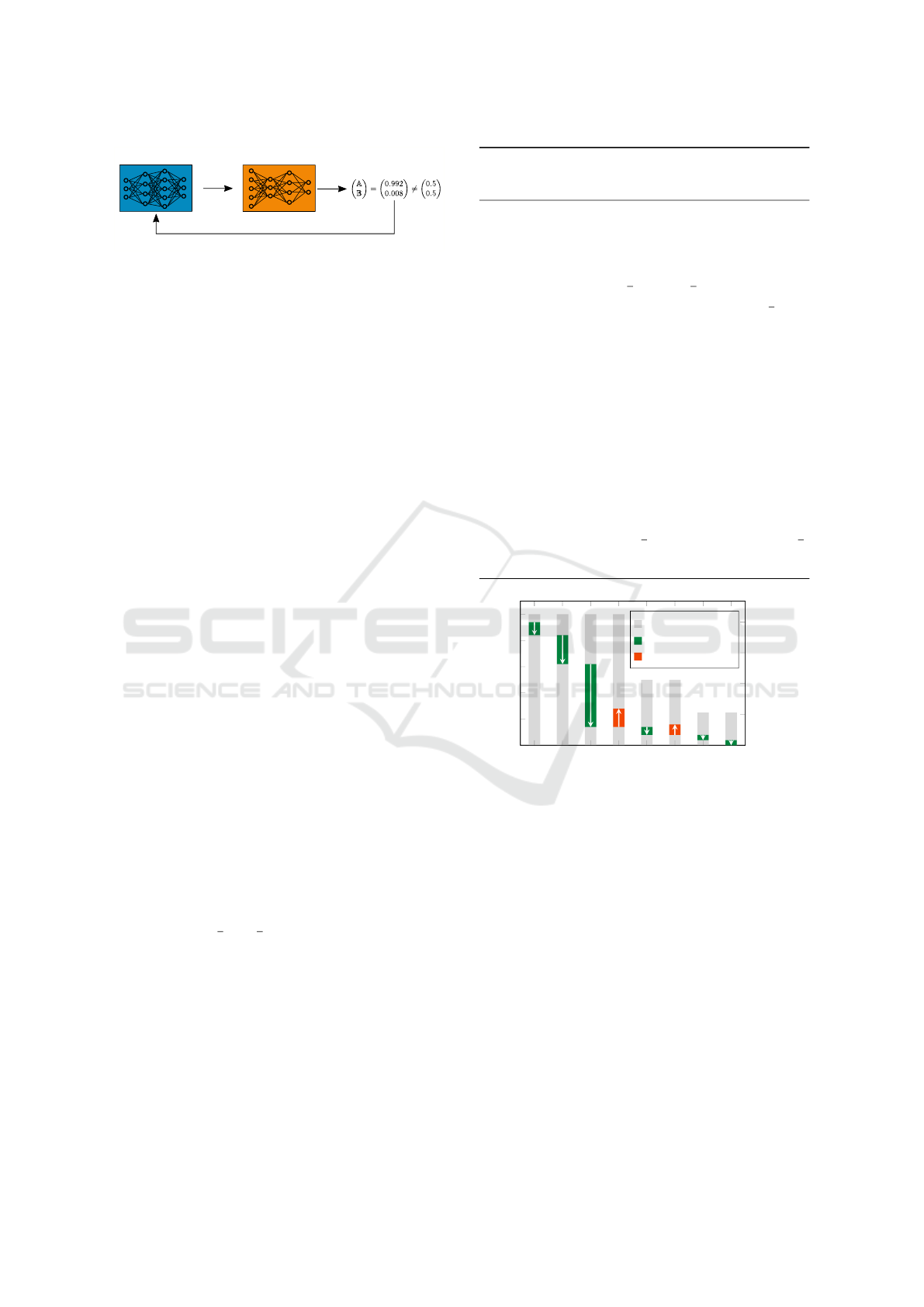
Figure 2: Property unlearning as a defense strategy against

PIAs.

sary as a preparation for protecting one’s own model,

the auxiliary data sets DS

and DS

can trivially

be subsets of the original training data of the target

model, since the model owner has access to the full

training data set. This yields a strong adversarial ac-

curacy as opposed to an outside adversary who might

need to approximate or extract this training data ﬁrst.

The same holds for white-box access to the model,

which is straightforward for the owner of a model.

Hence, the training of a reasonably good adversarial

meta classiﬁer A (> 99% accuracy) as a ﬁrst step of

property unlearning is easily achievable for the model

owner (see Sect. 5). As a second prerequisite, the tar-

get model M , which the owner wants to protect, also

needs to be fully trained with the original training data

set – having either property A or B.

To unlearn the property from M , we use back-

propagation. As in the regular training process, the

parameters of the target model M are modiﬁed by cal-

culating and applying gradients. But different from

original training, property unlearning does not opti-

mize M towards better classiﬁcation accuracy. In-

stead, the goal is to disable the adversary A from ex-

tracting the property A or B from M while keeping

its accuracy high.

In practice, the output of the adversarial meta-

classiﬁer A is a vector of length 2 (or: number of

properties k) which sums up to 1. Each value of the

vector corresponds to the predicted probability of a

property. As an example, the output [0.923,0.077]

means that the adversary A is 92.3% conﬁdent that

M has property A, and only 7.7% to have property B.

Thus, property unlearning aims to disable the adver-

sary from making a meaningful statement about M ,

i.e., an adversary output of [0.5,0.5] is pursued – or

more generally [

,...,

] for k properties.

Algorithm 1 shows pseudocode for the property

unlearning algorithm. The termination condition for

the while-loop in line 5 addresses the ability of the

adversary A: As long as A is signiﬁcantly more con-

ﬁdent for one of the properties, the algorithm needs

to continue. After calculating the gradients g au-

tomatically via TensorFlow’s backtracking algorithm

in line 6, the actual unlearning happens in line 7.

Here, the gradients are applied on the parameters

of model M , nudging them to be less property-

Algorithm 1: Property unlearning for a target model M , us-

ing property inference adversary A , initial learning rate lr,

and set of properties P = {A,B,...}.

1: procedure PROPUNLEARNING(M , A , lr, P)

2: k ← |P| ▷ number of properties (default 2)

3: Y ← A (M ) ▷ original adv. output |Y | = k

4: let i ∈ [k]

5: while ∃i : Y

≫

or Y

≪

6: g ← gradients for M s.t. ∀i : Y

→

7: M

′

← apply gradients g on M with lr

8: Y

′

← A (M

′

) ▷ update adversarial output

9: if ADVUTLT(Y

′

) < ADVUTLT(Y ) then

10: M ,Y ← M

′

11: else

12: lr ← lr/2 ▷ retry with decreased lr

13: end if

14: end while

15: return M

16: end procedure

17: function ADVUTLT(adv. output vector Y )

18: k ← |Y | ▷ number of properties (default 2)

19: return max

i∈[k]

(|Y

−

|) ▷ biggest diff. to

20: end function

1 2 3 4 5 6 7 8

2 · 10

−4

4 · 10

−4

6 · 10

−4

8 · 10

−4

learning rate

1 2 3 4 5 6 7 8

0.1

0.2

0.3

0.4

0.5

round of property unlearning

adversarial utility

learning rate

adv. util. decrease

adv. util. increase

Figure 3: A visualized example of the decreasing adver-

sarial utility during property unlearning with one adversary

for a single target model M . In each round, the adversar-

ial utility of M either decreases further towards the goal

of 0 (green bar), or the unlearning round is repeated with

a smaller learning rate (after a red bar). The ﬁnal result of

round 8 is a completely unlearned target model M with an

adversarial utility close to 0, see Algorithm 1.

revealing.

As described in Sect. 2.1, the learning rate con-

trols how much the gradients inﬂuence a single step.

If the parameters have been changed too much, the

current M

′

gets discarded and the gradients are reap-

plied with half the learning rate (see line 12 and vi-

sualization in Fig. 3). Reducing the learning rate to

its half has yielded the most promising results in our

experiments.

The effect of property unlearning in between

rounds of the algorithm is measured by the adversar-

SECRYPT 2023 - 20th International Conference on Security and Cryptography

316

ial utility, see lines 17–20. We calculate the adversar-

ial utility by analyzing the adversary output Y . Recall

that Y is a vector with k entries, with each entry Y

rep-

resenting the adversarially estimated probability that

the underlying training data set of the target model

M has property i. The adversarial utility is deﬁned

by the largest absolute difference of an entry Y

(see line 19). Remember that the goal of property un-

learning is to nudge the parameters of M such that the

output of the adversary is close to

for all k entries in

the output vector Y . The condition in line 9 therefore

checks whether the last parameter update from M to

′

was useful, i.e., whether the adversarial utility has

decreased. Only if this is the case, the algorithm gets

closer to the property unlearning goal. Otherwise, the

last update in M

′

is discarded and the next attempt is

launched with a lower learning rate. A visualization

of an exemplary run is given in Fig. 3.

5 PROPERTY UNLEARNING

EXPERIMENTS

To test property unlearning in practice, we have con-

ducted extensive experiments with different data sets.

Adversarial Property Inference Classiﬁer. As de-

scribed in Sect. 2.4, we use the attack approach

by (Ganju et al., 2018). This means that each instance

of an adversary A is an ANN itself, made up of mul-

tiple sub-networks φ and another sub-network ρ. Per

data set, we train one such adversarial meta classi-

ﬁer A , which is able to extract the respective proper-

ties A and B from a given target model.

Depending on the number of neurons in a layer of

the target model, our sub-NNs φ consist of 1–3 layers

of dense-neurons, containing 4–128 neurons each. In

the adversarial meta classiﬁer A , the number of layers

and number of neurons within the layers are propor-

tionate to the input size, i.e., the number of neurons

in the layer of the target model. These numbers are

evaluated experimentally, such that the meta classi-

ﬁers perform well, but do not offer more capacity than

needed (which would encourage overﬁtting).

Our sub-network ρ of A consists of 2–3 dense-

layers with 2–16 dense-neurons each. In our experi-

ments the output layer always contains two neurons,

one for each property A and B. For each of the three

data sets in the next section, we apply the following

steps to prepare for property unlearning:

• Design appropriate target model M for task.

• Extract two auxiliary data sets DS

and DS

for

each property A and B.

• Use each DS

and DS

as training data for 2000

shadow models. Shadow models have the same

architecture as the target model M .

• Design and train an adversarial meta classiﬁer A

on parameters of shadow models.

This adversarial model A may then be employed

in our property unlearning algorithm (see Sect. 4).

Data Sets and Network Architectures. We use

three different data sets to evaluate our approach, as

summarized in Table 1. For each data set and aux-

iliary data set DS

∗

, we train 2000 shadow models

and 2000 target models. For faster training and a

more realistic scenario, the auxiliary data sets DS

∗

are

smaller. While the shadow models are used to train

the adversaries A, the target models M are the sub-

jects of our experiments, i.e., we apply property un-

learning on these target models and measure the re-

sulting privacy-utility trade-off. The shadow models

and target models share the same architecture per data

set.

MNIST: is a popular database of labeled handwritten

digit images. As in (Ganju et al., 2018), we distort

all images with Gaussian noise (parameterized with

mean = 35, sd = 10) in a copy of the database. We

choose the property of having original pictures with-

out noise (A

MNIST

) and pictures with noise (B

MNIST

Our models for the MNIST classiﬁcation task are

ANNs with a preprocessing-layer to ﬂatten the im-

ages, followed by a 128-neurons dense-layer and a

10-neuron dense-layer for the output.

Census: is a tabular data set for income prediction.

The property inference attack aims at extracting the

ratio of male to female persons in the database, which

is originally 2:1. The auxiliary data set for prop-

erty A

Census

has a male:female ratio of 1:1,

Census

the original ratio of 2:1. The architecture of

the Census models consists of one 20-neurons dense-

layer and a 2-neurons output dense-layer.

UTKFace: contains over 23000 facial images. We

choose gender recognition as the task for the target

models M . Concerning our choice of properties,

we create a data set consisting only of images with

ethnicity White from the original data set for prop-

erty A

UTK

. The data set for property B

UTK

is com-

prised of images labeled with Black, Asian, Indian,

and Others.

For UTKFace gender recognition, we use a convo-

lutional neural network (CNN) architecture with three

sequential combinations of convolutional, batch nor-

malization, max-pooling and dropout layers, leading

to one dense-layer with 2 neurons.

Lessons Learned: Defending Against Property Inference Attacks

317

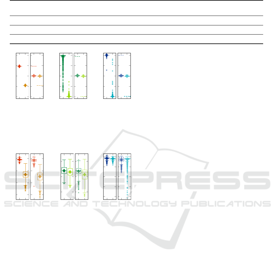
Table 1: The data sets used for the experiments. init.=initial, distrib.=distribution.

Experiment Data set Size Target Property |DS

∗

Shadow model

accuracy

Init. PIA

accuracy

MNIST

(LeCun et al., 1998) 70K Gaussian noise 12K 88.3–94.5% 100%

Census

Census Income Data Set 48K gender distrib. 15K 84.7% 99.3%

UTK

(Zhang et al., 2017) 23K race distrib. 10K 88.0–88.3% 99.8%

A B

0.25

0.5

0.75

output of adversary A

MNIST

A B

0.25

0.5

0.75

(a) E

MNIST

A B

0.25

0.5

0.75

output of adversary A

Census

A B

0.25

0.5

0.75

(b) E

Census

A B

0.25

0.5

0.75

output of adversary A

UTK

A B

0.25

0.5

0.75

UTK

Figure 4: Each experiment before and after property un-

learning, depicting the certainty of adversary A in classify-

ing A and B. The dashed lines represent the avg. accuracy

before property unlearning was applied on 2000 target mod-

els.

A B

0.8

0.85

0.9

0.95

task accuracy of M

MNIST

A B

0.8

0.85

0.9

0.95

(a) E

MNIST

A B

0.82

0.84

0.86

task accuracy of M

Census

A B

0.82

0.84

0.86

(b) E

Census

A B

0.5

0.6

0.7

0.8

0.9

task accuracy of M

UTK

A B

0.5

0.6

0.7

0.8

0.9

UTK

Figure 5: Each experiment before and after property un-

learning regarding the accuracy loss of the target models

M . The dashed lines represent the average accuracy val-

ues before property unlearning was applied on 2000 target

models.

5.1 Experiment 1: Property unlearning

In this section we experimentally evaluate the per-

formance of property unlearning to defend against a

speciﬁc PIA adversary. For each of the data sets de-

scribed above, we have trained 2000 test models in

the same way we have created the shadow models.

We refer to these test models as target models.

The ﬁgures in this section contain boxplot-graphs.

Each boxplot consists of a box, which vertically spans

the range between the ﬁrst quartile Q

and the third

quartile Q

, i.e., the range between the median of the

upper and lower half of the data set. The horizon-

tal line in a box marks the median and the diamond

marker indicates the average value.

MNIST. For the MNIST experiment E

MNIST

, the

adversary classiﬁes the properties A and B with

high certainty in all instances before unlearning, see

Fig. 4a. After unlearning, the adversary cannot in-

fer the property of any of the MNIST target mod-

els M

MNIST

– as intended. Meanwhile, the accuracy

of the target models M

MNIST

decreased slightly from

an average of 94.6% by 0.4%P to 94.2% for models

with property A, respectively from 88.3% by 0.8%P

to 87.5% for models with property B (see Fig. 5a).

Recall that property B was introduced by applying

noise to the training data, hence the affected models

perform worse in general.

Census. Property unlearning was also successfully

applied in the E

Census

experiment to harden the tar-

get models M

Census

against a PI adversary A

Census

, see

Fig. 4b. Note that the performance of A

Census

is not

ideal for property A, classifying some of the instances

incorrectly. However, 99.3% of the 2000 instances

were classiﬁed correctly by the adversary before prop-

erty unlearning. As desired, the output of A

Census

centered around 0.5 for both properties after property

unlearning. The magnitude of the target models’ ac-

curacy loss is small, with an average drop of 0.1%P

for property A (84.8% to 84.7%) and 0.3%P (84.6%

to 84.3%) for property B, see Fig. 5b.

UTKFace. In the E

UTK

experiment, property un-

learning could be successfully applied to all mod-

els (see Fig. 4c) to harden the target models against

PIAs. On average, the accuracy of the target models

dropped by 1.3%P (from 88.2% to 86.9%) for mod-

els trained with the data set DS

and by 0.1%P (from

87.9% to 87.8%) for target models trained with DS

see Fig. 5c. This yields an average accuracy drop of

0.8%P across the target models for both properties

(from 88.1% to 87.3%).

5.2 Experiment 2: Iterative Property

Unlearning

In the previous section, the results of Experiment 1

have shown that property unlearning can harden a

target model M against a single PI adversary, i.e.,

a speciﬁc adversarial meta classiﬁer A (see Figure

2). The setup of Experiment 2 aims to improve

that by generalizing the unlearning. Therefore, the

same target model M is unlearned iteratively against

SECRYPT 2023 - 20th International Conference on Security and Cryptography

318

backpropagation

train

backpropagation

train

...

test

...

Figure 6: In reference to Fig. 2, iterative property unlearn-

ing works by performing single property unlearning for n

different adversarial meta classiﬁer instances A iteratively

on a target model M

(0)

. The resulting target model M

(n)

then evaluated by additional m instances of A.

a range of different adversary instances A (see Fig-

ure 6). The results of our experiments are based

on 200 target models. We unlearn each initial tar-

get model M

(0)

iteratively for n different adversar-

ial meta classiﬁers A

, where n = 15. After that,

the resulting iteratively unlearned target model M

(n)

is tested by another distinct adversarial meta clas-

siﬁer. To increase the signiﬁcance of our results,

we choose to test the resulting target model M

(n)

with m = 5 additional distinct adversarial meta classi-

ﬁers. Furthermore, we apply a 4-fold cross validation

technique to this constellation of in total 20 distinct

adversarial classiﬁers. Finally, the results are plot-

ted in boxplots similar to Experiment 1: Here, each

boxplot is visualizing 200 (target models) ∗4 (folds) ∗

5 (adversary outputs in a fold) = 4000 data points.

The shadow models which were used to train the

20 adversaries A have been grouped such that the 5

testing adversaries’ training set is disjunct from the

training set of the 15 adversaries used for unlearn-

ing. The order of the 15 adversaries for unlearning

has been chosen randomly for each of the 200 target

models M .

The overall results on the MNIST data set in Fig-

ure 7 show the iterative unlearning process for prop-

erty A and B. Each column on the x-axis represents

an iteration step of the iterative unlearning procedure.

On the y-axis, the prediction of the adversary regard-

ing the corresponding property is plotted, which is

ideal for property A and B to be 0 and 1, respectively.

The goal of property unlearning is y = 0.5, such that

the attacker is not able to distinguish the property.

Clearly, the second column shows that after applying

property unlearning once, a distinct adversary, i.e.,

not the adversary which was involved in the unlearn-

ing process, is still able to infer the correct property

for most target models M . The plots show that after

about ten iterations of property unlearning, the aver-

age output of the 5 testing adversaries converges to-

wards an average of prediction probability 0.5 (for

both properties A and B). While this could be mis-

interpreted as ultimately reaching the goal of prop-

1 2 3 4 5 6 7 8 9 10 11 12 13 14 15 16

0.5

output of adversaries A

MNIST

1 2 3 4 5 6 7 8 9 10 11 12 13 14 15 16

0.5

Figure 7: Results of iterative unlearning experiment for

property A (left) and B (right). For each of the 200 tar-

get models M , the predictions of all 5 testing adversaries

are plotted along the y-axis before unlearning (ﬁrst column)

and after each unlearning iteration (other 15 columns).

2 4

0.5

output of adversaries A

MNIST

(a)

2 4

0.5

(b)

2 4

0.5

(c)

2 4

0.5

(d)

Figure 8: Individual adversary outputs after all 15 unlearn-

ing iterations for property A target models. Recall that be-

fore unlearning, all adversaries have correctly inferred prop-

erty A by outputting y = 0.

erty unlearning, we introduce Figure 8 which paints a

more ﬁne-grained picture of the last column of Figure

7. Here, each of the four plots contain ﬁve indepen-

dent boxplots corresponding to the ﬁve distinct test

adversaries in one fold of the cross validation process.

Each boxplot presents the prediction results of one

adversary for the 200 independently unlearned target

models M

(15)

of the experiment.

While the plots of Figure 7 suggest that the adver-

saries’ outputs are evenly spread across the interval

[0,1] with both an average and median close to 0.5,

Figure 8 shows that this is only true for the indistinct

plot of all 4 experiments with 5 testing adversaries

each. We want to point out three key observations:

1. Most adversaries do not have median outputs near

0.5 after 15 unlearning iterations.

2. For some adversary instances A, target models

have been “over-unlearned” by the 15 iterations with

their output clearly nudged into opposite of their orig-

inal output, e.g., adversary 3 in Fig. 8d.

3. Most importantly, other adversaries are still cor-

rectly inferring the property for most or even all

200 target models with high conﬁdence after the 15

unlearning iterations, e.g., the second adversary in

Fig. 8a.

Lessons Learned: Defending Against Property Inference Attacks

319

5.3 Experiment Discussion

Recall our goal for property unlearning: We want to

harden target models in a generic way, such that arbi-

trary PI adversaries are not able to infer pre-speciﬁed

properties after applying property unlearning.

Experiment 1 (single property unlearning) shows

that property unlearning is very reliable to harden tar-

get models against speciﬁc adversaries. However, Ex-

periment 2 (iterative property unlearning) indicates

that single property unlearning fails to generalize, i.e.,

protect against all PI adversaries of the same class.

This is shown in Experiment 2 by putting each tar-

get model through 15 iterations of property unlearn-

ing with one distinct adversary per iteration. After

this, some adversaries are still able to infer the orig-

inal properties of all target models (see third key ob-

servation in Sect. 5.2). This means that in the worst

case, i.e., for the strongest adversaries, 15 iterations

of property unlearning do not sufﬁce – while for other

(potentially weaker) adversaries, 15 or even less iter-

ations are enough to harden the models against them.

In conclusion, property unlearning does not meet our

goal of being a generic defense strategy, i.e., protect-

ing against a whole class of adversaries instead of a

speciﬁc adversary.

6 EXPLAINING PI ATTACKS

To explore the reasons behind this limitation of

property unlearning, we use the explainable AI tool

by (Ribeiro et al., 2016): LIME (Local Interpretable

Model-agnostic Explanations) allows to analyze deci-

sions of a black-box classiﬁer by permuting the values

of its input features. By observing their impact on the

classiﬁer’s output, LIME generates a comprehensible

ranking of the input features.

Recall that in the previous experiment (Sect. 5.2),

we have seen that adapting the weights of a target

model M s.t. an adversarial meta-classiﬁer A

can-

not launch a successful PIA does not defend against

another adversarial meta-classiﬁer A

trained for the

same attack. Therefore, we use LIME to see whether

different meta-classiﬁers A

and A

rely on the same

weights of a target model M to infer A or B.

For comprehensible results, we use LIME images.

We convert the trained parameters of an MNIST tar-

get model M into a single-dimensional vector with

length 101 770, so LIME can interpret them as an

image. For segmentation, we use a dummy algo-

rithm which treats each weight of M (resp. pixel)

as a separate segment of the ’image’. This is nec-

essary because unlike in an image, neighboring ’pix-

Figure 9: LIME produced, partial heat maps of different

meta-classiﬁer instances A

and A

for the same MNIST

target model M . Dark pixels represent parameters with

high impact on the decision of A, yellow pixels imply a

low impact.

els’ of M ’s weights do not necessarily have semantic

meaning. For reproducible and comparable results,

we have initialized all LIME instances with the same

random seed.

LIME Results. We have instantiated LIME with two

property inference meta-classiﬁers A

and A

to ex-

plain their output for the same MNIST target model

instance M . The output of LIME is a heat map rep-

resenting the weights and biases of M , see Fig. 9.

For practical reasons, we have only visualized the ﬁrst

784 pixels of the heat map and transformed them to

a two-dimensional space. Although A

and A

are

trained in the same way and with the same shadow

models (see Sect. 5), the two heat maps for classifying

the property of the same target model M in Fig. 9 are

clearly different: While some of M ’s weights have

similar importance, i.e., the heat map pixels have a

similar color, many weights have very different im-

portance for the two adversarial meta classiﬁers A

and A

To understand why meta-classiﬁers can rely on

different parts of target model parameters to infer a

training data property, we analyze the parameter dif-

ferences induced by such properties on an abstract

level.

t-SNE (t-Distributed Stochastic Neighbor Embedding

(Van der Maaten and Hinton, 2008)) is a form of di-

mensionality reduction which is useful for clustering

and visualizing high-dimensional data sets. In partic-

ular, the algorithm needs no other input than the data

set itself and some randomness.

In the t-SNE experiment, the input data set is

comprised of the trained weights and biases of the

shadow models. We apply this to the three data sets

MNIST, Census and UTKFace. As before, we use

2000 shadow models (1000 with property A and 1000

with property B). Our goal is revealing to which ex-

tend the trained parameters are inﬂuenced by a statis-

tical property of the training data set. In particular,

if the data agnostic approach t-SNE is able to cluster

models with different properties apart, we can assume

the inﬂuence of a property on model parameters to be

signiﬁcant.

t-SNE Results. As depicted in Fig. 10, t-SNE has

produced a well deﬁned clustering for the two image

SECRYPT 2023 - 20th International Conference on Security and Cryptography

320

Figure 10: t-SNE visualization of MNIST (left), Census

(center) and UTKFace (right) models. Each yellow dot rep-

resents a model with property A, each purple dot a B model.

data sets MNIST and UTKFace: models trained with

property A training data sets (yellow dots) are placed

close to the center of the visualization, while prop-

erty B models (purple dots) are mostly further from

the center. This indicates that the properties, deﬁned

in Sect. 5 for MNIST and UTKFace, heavily inﬂu-

ence the weights and biases of the trained models.

In fact, without any additional information about the

parameters or the properties of the underlying train-

ing data sets, t-SNE is able to distinguish the models

by property with surprisingly high accuracy. Based

on these results, one could construct a simple PI ad-

versary A

t-SNE

by measuring the euclidean distance ℓ

of a target model from the center of the t-SNE clus-

tering. If ℓ is below a certain threshold for a target

model M , A

t-SNE

infers property A, otherwise it in-

fers property B. For MNIST, A

t-SNE

has 86.7% ac-

curacy based on our experiment, while the UTKFace

t-SNE

has 72.0% accuracy. We stress that these two

t-SNE

are solely based on the t-SNE visualization of

the model parameters, no training on shadow models

is needed.

However for Census, t-SNE has not clustered

models with different properties of their training data

sets apart (see second visualization in Fig. 10). In

contrast to the other two data sets MNIST and UTK-

Face, Census is a tabular data set. It also may be that

the properties deﬁned in Sect. 5 have a smaller immi-

nent impact on the weights and biases during train-

ing. We leave a more profound analysis of possible

reasons for the different behavior of the t-SNE visu-

alization on the three data sets for future work.

7 DISCUSSION

We now discuss our results to yield insights for fu-

ture research in the yet unexplored ﬁeld of defending

against PIAs.

Choosing the Right Defense Approach. We have

introduced defense mechanisms at different stages

of the ML pipeline. Both property unlearning ex-

periments are positioned after the training and be-

fore its prediction phase, respectively its publica-

tion. In contrast, the preprocessing approach is ap-

plied prior to the training. Since most ML algorithms

require several preprocessing steps, implementing a

defense mechanism based on preprocessing training

data could be easily adapted in real-world scenar-

ios. At least for tabular data, our preprocessing ex-

periments (see full paper (Stock et al., 2022)) have

shown a good privacy-utility trade-off, especially the

artiﬁcial data approach. Nevertheless, depending on

the organization and application scenario of a ML

model, a post-training approach like property unlearn-

ing might have its beneﬁts as well. Further exper-

iments could test the combination of both pre- and

post-training approaches. Since both of them are

not promising to provide the generic PIA defense we

aimed for, we assume the combination of both does

not signiﬁcantly improve the defense. Instead, we

suggest to focus further analyses on other approaches

during the training, as laid out in Sect. 8.

Lessons Learned. With our cross-validation exper-

iment in Sect. 5.2, we have shown how PI adver-

saries react to property unlearning in different ways.

Some adversaries could still reliably infer training

data properties after 15 property unlearning iterations,

while other adversaries reliably inferred the wrong

property after the same process. This shows that it is

hard to utilize a post-training technique like prop-

erty unlearning as a generic defense against a whole

class of PI adversaries: After all, one needs to de-

fend against the strongest possible adversary while

simultaneously being careful not to introduce addi-

tional leakage by adapting the target model too much.

Depending on the adversary instance, most of our tar-

get models clearly show one of these deﬁciencies after

15 rounds of property unlearning.

Our t-SNE experiment in Sect. 6 shows that at

least for image data sets, statistical properties of

training data sets have a severe impact on the

trained parameters of a ML model. This is in line

with the LIME experiment, which shows how two PI

adversaries with the same objective focus on differ-

ent parts of target model parameters. If a property

is manifested in many areas of a model’s parameters,

PI adversaries can rely on different regions. This im-

plies that completely pruning such properties from a

target model after training is hard to impossible, with-

out severely harming its utility.

8 FUTURE WORK

Preprocessing Training Data. We have not tested

training data preprocessing in an adaptive environ-

ment yet, where the adversary would adapt to the pre-

Lessons Learned: Defending Against Property Inference Attacks

321

processing steps and retrain on shadow models with

preprocessed training data as well. Intuitively, this

would weaken the defense while costing the same

utility in the target models. Additionally, as the tech-

nique with most potential for defending against PIAs

for tabular data, the generation of artiﬁcial data could

be further explored: One could adapt the synthesis al-

gorithm s.t. statistical properties are arbitrarily mod-

iﬁed in the generated data set. A similar goal is pur-

sued in many bias prevention approaches in the area

of fair ML.

Adapting the Training Process. Another method

from a similar area called fair representation learning

is punishing the model when learning biased informa-

tion by introducing a regularization term in the loss

function during training, e.g., (Creager et al., 2019).

As a defense strategy against PIAs, one would need

to introduce a loss term which expresses the current

property manifestation within the model and causes

the model to hide this information as good as possible.

In theory, this would be a very efﬁcient way to pre-

vent the property from being embedded in the model

parameters. Since it would be incorporated into the

training process, the side effects on the utility of the

target model should be low.

Post-Training Methods. (Liu et al., 2022) experi-

ment with knowledge distillation (KD) as a defense

against privacy attacks like membership inference.

The idea is to decrease the number of neurons in an

ANN in order to lower its memory capacity. Unfortu-

nately, the authors do not consider PIAs – it would be

interesting to see the impact of KD on their success

rate.

9 CONCLUSION

In this paper, we performed the ﬁrst extensive anal-

ysis on different defense strategies against white-box

property inference attacks. This analysis includes a

series of thorough experiments on property unlearn-

ing, a novel approach which we have developed as a

dedicated PIA defense mechanism. Our experiments

show the strengths of property unlearning when de-

fending against a dedicated adversary instance and

also highlight its limits, in particular its lacking abil-

ity to generalize. We elaborated on the reasons of this

limitation and concluded with the conjecture that sta-

tistical properties of training data are deep-seated in

the trained parameters of ML models. This allows PI

adversaries to focus on different parts of the param-

eters when inferring such properties, but also opens

up possibilities for much simpler attacks, as we have

shown via t-SNE model parameter visualizations.

Apart from the post-training defense property un-

learning, we have also tested different training data

preprocessing methods (see full paper version (Stock

et al., 2022)). Although most of them were not di-

rectly targeted at the sensitive property of the training

data, some methods have shown promising results. In

particular, we believe that generating a property-free,

artiﬁcial data set based on the distribution of an orig-

inal training data set could be a candidate for a PIA

defense with very good privacy-utility tradeoff.

ACKNOWLEDGEMENTS

We wish to thank Anshuman Suri for valuable discus-

sions and we are grateful to the anonymous reviewers

of previous versions of this work for their feedback.

REFERENCES

Ateniese, G., Mancini, L. V., Spognardi, A., Villani, A.,

Vitali, D., and Felici, G. (2015). Hacking smart ma-

chines with smarter ones: How to extract meaningful

data from machine learning classiﬁers. IJSN.

Creager, E., Madras, D., Jacobsen, J.-H., Weis, M., Swer-

sky, K., Pitassi, T., and Zemel, R. (2019). Flexibly fair

representation learning by disentanglement. In ICML.

Dwork, C., McSherry, F., Nissim, K., and Smith, A. (2006).

Calibrating noise to sensitivity in private data analysis.

In TCC.

Fredrikson, M., Jha, S., and Ristenpart, T. (2015). Model

inversion attacks that exploit conﬁdence information

and basic countermeasures. In CCS.

Ganju, K., Wang, Q., Yang, W., Gunter, C. A., and Borisov,

N. (2018). Property inference attacks on fully con-

nected neural networks using permutation invariant

representations. In CCS.

LeCun, Y., Bottou, L., Bengio, Y., and Haffner, P. (1998).

Gradient-based learning applied to document recogni-

tion. IEEE.

Liu, Y., Wen, R., He, X., Salem, A., Zhang, Z., Backes,

M., Cristofaro, E. D., Fritz, M., and Zhang, Y. (2022).

ML-Doctor: Holistic risk assessment of inference at-

tacks against machine learning models. In USENIX

Security.

Mahloujifar, S., Ghosh, E., and Chase, M. (2022). Property

inference from poisoning. In S&P.

Melis, L., Song, C., De Cristofaro, E., and Shmatikov, V.

(2019). Exploiting unintended feature leakage in col-

laborative learning. In S&P.

Nasr, M., Shokri, R., and Houmansadr, A. (2018). Machine

Learning with Membership Privacy using Adversarial

Regularization. In CCS.

Papernot, N., McDaniel, P., Goodfellow, I., Jha, S., Celik,

Z. B., and Swami, A. (2017). Practical black-box at-

tacks against machine learning. In ASIACCS.

SECRYPT 2023 - 20th International Conference on Security and Cryptography

322

Ribeiro, M. T., Singh, S., and Guestrin, C. (2016). Why

should i trust you? explaining the predictions of any

classiﬁer. In SIGKDD.

Rigaki, M. and Garcia, S. (2020). A survey of privacy at-

tacks in machine learning. Arxiv.

Shokri, R., Stronati, M., Song, C., and Shmatikov, V.

(2017). Membership inference attacks against ma-

chine learning models. In S&P.

Song, C., Ristenpart, T., and Shmatikov, V. (2017). Machine

learning models that remember too much. In CCS.

Song, C. and Shmatikov, V. (2020). Overlearning Reveals

Sensitive Attributes. In ICLR.

Song, L. and Mittal, P. (2021). Systematic evaluation of

privacy risks of machine learning models. In USENIX

Security.

Stock, J., Wettlaufer, J., Demmler, D., and Federrath, H.

(2022). Lessons learned: Defending against property

inference attacks. arXiv preprint arXiv:2205.08821.

Suri, A., Kanani, P., Marathe, V. J., and Peterson, D. W.

(2022). Subject membership inference attacks in fed-

erated learning. Arxiv.

Tang, X., Mahloujifar, S., Song, L., Shejwalkar, V., Nasr,

M., Houmansadr, A., and Mittal, P. (2021). Mitigat-

ing membership inference attacks by self-distillation

through a novel ensemble architecture. USENIX Sec.

Van der Maaten, L. and Hinton, G. (2008). Visualizing data

using t-SNE. JMLR.

Zhang, W., Tople, S., and Ohrimenko, O. (2021). Leakage

of dataset properties in multi-party machine learning.

In USENIX Security.

Zhang, Z., Song, Y., and Qi, H. (2017). Age pro-

gression/regression by conditional adversarial autoen-

coder. In CVPR.

Lessons Learned: Defending Against Property Inference Attacks

323