Exploring Functional Patterns of Driving Records by Interacting with

Major Classes and Territory Using Generalized Additive Models

Shengkun Xie

, Anna T. Lawniczak

and Clare Chua-Chow

Global Management Studies, Ted Rogers School of Management, Toronto Metropolitan University, Toronto, Canada

Department of Mathematics and Statistics, University of Guelph, Guelph, Canada

Keywords:

Generalized Additive Models, Rate-Making, Insurance Rate Regulation, Business Data Analytics.

Abstract:

Studying the safe driver index, such as Driving Records (DR), is essential to auto insurance regulation. Part

of the auto insurance regulation aims to estimate the relativity of major risk factors, including DR, to provide

some benchmark values for auto insurance companies. The risk relativity estimate of DR is often through

either an assessment via empirical loss cost or a statistical modelling approach such as using generalized

linear models. However, these methods are only able to give an estimate on an integer level of DR. This work

proposes a novel approach to estimating the risk relativity of DR via generalized additive models (GAM).

This method makes the integer level of DR continuous, making it more ﬂexible and practical. Extending the

generalized linear model to GAM is critical as investigating this new method could enhance applications of

advanced statistical methods to the actuarial practice. Thus, making the proposed methodology of analyzing

the safe driver index more statistically sound. Furthermore, exploring functional patterns by interacting with

major classes or territories allows us to ﬁnd statistical evidence to justify the existence of correlations between

risk factors. This may help address the issue of potential double penalties in insurance pricing and call for a

solution to overcome this problem from a statistical perspective.

1 INTRODUCTION

Risk factors play a major role in both auto insurance

pricing and rate regulation (Xie, 2021). Major risk

factors used in rate regulation may include Driving

Record (DR), Territory, and Type of Use (i.e., Class)

(Xie and Lawniczak, 2018). The major risk factors

are critical variables that can be used for this pur-

pose, and investigating these factors allows us to bet-

ter understand their key characteristics. From a reg-

ulation perspective, it is important to ensure that the

used model, the modelling process and their valida-

tion processes meet the requirements of regulatory

rules. It is also crucial for transparency that the pub-

lic know what driving characteristics affect the pre-

miums they pay. Although not always possible, insur-

ance companies try to set premiums based on risk fac-

tors and they may adjust premiums based on the loss

cost from preceding years after the review by regula-

tors. Changes in risk affect the premiums that auto

insurance companies charge and they are reﬂected in

the premiums drivers pay. However, drivers may see

these changes in premiums as discriminatory or unfair

because they need to be made aware of the insurers’

perception of risk variation. On the other hand, ex-

amining certain risk factors’ roles in affecting relativ-

ity also helps improve auto insurance fairness. This

is because risk classiﬁcation of these factors needs

to be accurate for insurers to properly charge the in-

sured; otherwise, some will be overcharged, and oth-

ers will be undercharged. Identifying how auto insur-

ance companies classify risk by examining how rel-

ativity changes when we include certain risk factors

such as Type of Use gives the public more information

about how premiums are set (Abraham, 1985). This

increase in awareness allows more drivers to perceive

premiums as being fair from actuarial perspectives

(Meyers and Van Hoyweghen, 2018; Landes, 2015;

Frezal and Barry, 2020).

Many factors directly cause car accidents, such as

cell phone use, drug use, or alcohol use (Rolison et al.,

2018). They are considered as impaired driving when

a car accident happens, and there is a strong cause-

and-effect relationship between these factors and car

accidents. In auto insurance, a Driving Record (DR)

is created to represent a given driver’s accident his-

tory and this record is indicative of causing the in-

surance losses. Therefore, DR as a safe driver index

Xie, S., Lawniczak, A. and Chua-Chow, C.

Exploring Functional Patterns of Driving Records by Interacting with Major Classes and Territory Using Generalized Additive Models.

DOI: 10.5220/0012068900003541

In Proceedings of the 12th International Conference on Data Science, Technology and Applications (DATA 2023), pages 271-278

ISBN: 978-989-758-664-4; ISSN: 2184-285X

 2023 by SCITEPRESS – Science and Technology Publications, Lda. Under CC license (CC BY-NC-ND 4.0)

271

(Brown et al., 2004) plays a crucial role in auto insur-

ance pricing. In Canada, DR has 7 levels correspond-

ing to how many years a driver has not been involved

in a car accident. For example, when DR equals zero,

there are zero years that this driver has had no acci-

dent. This may imply that this driver recently had a

car accident or is a new driver with zero years of driv-

ing history. Because of this implication, for drivers

with a low driving record and no accident history, the

insurance premium may be double-penalized as other

risk factors are used to indicate a similar level of risk,

such as young driver class or a low number of years

of having a driver’s license. This may call for applica-

tion of statistical methods that can help to reveal the

potential interactions among risk factors more accu-

rately. From the statistical modelling point of view,

this may imply that modelling or analysis of loss data

may need to be conditioned on a certain level of an-

other risk factor. For example, the DR pattern may

depend on a level of Class (i.e., Type of Use) or a ter-

ritory level.

To better understand the relationship between in-

surance loss and considered risk factors, ﬁrst, we ex-

amine the functional pattern of DR using general-

ized additive models (GAM) (Hastie, 2017; Wood,

2006). The GAM is an extension of generalized linear

models (GLM) that allows for ﬂexibility by having

the response variable to be linear but explained using

functions that can uncover non-linear relationships

between the independent variables and its response

variable. GAM has been recently applied to auto in-

surance pricing, particularly for modelling telematics

data (Huang and Meng, 2019; Boucher et al., 2017;

Meng et al., 2022). The GAM constructed by us in

this paper was then extended by adding the Class fac-

tor of the driver and the Territory factor. The Class

factor has 14 different categorical levels and the Terri-

tory factor has 2 different levels, rural or urban. Class

and Territory are model factors in GAM which pro-

duce a separate smooth term for each level of Class

and Territory. Within this GAM modelling frame-

work, we combine two separate models that use loss

cost and premium as response variables into one. This

combination is possible because, when modelling loss

cost and premium, they are assumed to have the same

set of predictors. This combination of loss cost and

premium as a model response is particularly novel in

actuarial data analysis and it allows an overall better

estimate of risk factor relativities.

Furthermore, in this work, we propose using

GAM as an alternative approach to estimating DR

relativities, often derived from GLM in current actu-

arial practice (Ohlsson and Johansson, 2010). This

new method can help to de-couple the correlation be-

tween different risk factors and to avoid the double

penalty in auto insurance pricing when using multi-

plicative pricing algorithms. The obtained functional

patterns from GAM lead to a better understanding of

DR characteristics and how they are affected by other

major risk factors. The proposed method maintains

the model interpretability while sharing some power

from the machine learning approaches (Burka et al.,

2021; Denuit et al., 2021) by providing us with an

estimate of non-linear functional patterns of DR.

2 MATERIALS AND METHODS

2.1 Data

The data used in this paper comes from the Insur-

ance Bureau of Canada (IBC). The data sets con-

sist of aggregated loss costs, premiums, and expo-

sures used to calculate risk relativity for each driving

record level, class and other major risk factors. Loss

cost is deﬁned as total losses (claim amount and ex-

penses used for settling claims) divided by the total

number of exposures. The premiums are the average

earned premiums. To systematically analyze loss cost

and premium, we deﬁne a dummy variable to indi-

cate whether the value for a particular combination of

driving record and class is the average loss cost (pure

premium) or average premium (rate). The value 1 in-

dicates that it is loss cost, and 0 means it is premium.

The response variable is denoted by LOSSPREM, and

its observation consists of loss cost or premium, de-

pending on which case. The data also are separated

by territory, rural or urban, where 1 indicates that it

corresponds to urban and 0 represents the rural area.

There are 3 major coverages that we focus on, Acci-

dent Beneﬁt (AB), Collision (COL), and Third Party

Liability (TPL). Each coverage has three years of data

from 2009 to 2011, and we also include a summarized

data set that combines all three years. Exposures are

taken as weights for DR and Class to produce accu-

rate conﬁdence intervals.

2.2 Extending GLM to GAM

As we mentioned earlier, the traditional approach to

estimating the risk relativity of each level of a given

risk factor is either through empirical measures based

on the relative level of loss costs or via a modelling

approach that includes a set of risk factors as inde-

pendent variables and the loss cost as the response

for some statistical models such as generalized lin-

ear models. However, the empirical measures of the

relative loss cost level for each combination of fac-

DATA 2023 - 12th International Conference on Data Science, Technology and Applications

272

Table 1: Deﬁnitions of four major classes used in this work. Note, the risk exposures for these four classes account for 92%

of the total risk exposures (i.e., the total number of vehicles per accident year).

Class 1 Principal operator is 25 years of age or over. Class 3 Principal operator is 25 years of age or over

No male driver under is 25 years of age; No male drivers are under 25 years of age.

no female drivers are under 25 years of age (not Automobile is used for business.

having a spouse or same-sex partner), Maximum 25% is used for business.

without driver training.

Not more than 2 drivers, per automobile, are in

the household, each of whom has held a

valid driver’s license for the past 3 years.

Class 2 Principal operator is 25 years of age or over. Class 7 No male drivers are under 25 years of age.

No male driver is under 25 years of age; no

female drivers are under 25 years of age (not

having a spouse or same-sex partner),

without driver training.

tor level can only serve as some benchmark values as

they lack statistical powers, which can be used to cap-

ture the randomness of loss cost. One of the problems

with using generalized linear models is that the esti-

mated risk relativities of DR may not be monotonic,

and this may further affect the stability of benchmark

values when it comes to regulation. In rate regula-

tion, the relativity of DR at each level must decrease

monotonically with the increase of years of no claims,

which takes values 0, 1, 2, . . ., but there is no guar-

antee of this required functional pattern when using

GLM modelling. The monotonic function of DR is

required, but the empirical estimate from the yearly

data does not guarantee this functionality. The GAM

model can assist in a better estimate of the overall pat-

tern of DR concerning the number of years without

accidents. To ensure a monotonic DR pattern, we ﬁt

the data to a generalized additive model (GAM) in-

stead, which is given as follows:

jlm

= γ

0 jlm

+ s(DR) + γ

1 j

Class

Territory

+ γ

Source

+ ε

jlm

, (1)

where s() is a monotonic spline function used to es-

timate the relationship between DR and the response

variable, i.e. LOSSPREM, denoted by Y . γ and ε

stand for the model coefﬁcients and model error, re-

spectively. k indicates which combination of accident

year and major coverage is considered. j indicates the

jth level of Class , l shows the lth level of Territory

and m indicates if it is for loss cost or premium. Using

GAM modelling, we impose the functionality of DR

with respect to the number of years of no accidents.

These splines are ﬂexible functions that allow us to

model non-linear relationships as they determine the

shape of the trend to ﬁt the data. Knots are the number

of joins for two or more polynomial basis curves. The

number of knots or the basis complexity chosen was

cross-validated, and it was selected as 5 in this work.

The R package used was ”mgcv”, and the monotonic

cubic spline was used to estimate the functional pat-

terns. This is considered a constrained spline for re-

gression problems. The log link function was used to

transform the response, and for all models, the error ε

in (1) is assumed to be Gamma distributed, the most

common distribution for auto insurance loss.

Another important aspect of estimating relativi-

ties for risk factors is to consider the interaction be-

tween different risk factors. For instance, in Figure

1, we show how loss cost patterns by DR interact

with Class and Territory variables. The curves inter-

act among levels of territory, particularly for Rural.

This may suggest that DR patterns depend on the lev-

els of Class and Territory. On the other hand, DR

patterns measured by premiums show that the inter-

action has been eliminated to some extent. There-

fore, including premium data in modelling will help

guide the estimate of relativity in the desired direction

to reduce the variability associated with the estimate.

However, in actuarial practice, it is not easy to incor-

porate excessive interactions to the model as consid-

ering too many interactions among different factors

will signiﬁcantly decrease the number of exposures

associated with each interaction. This may further

cause the credibility of the estimated coefﬁcient in the

model. To overcome this difﬁculty and improve the

interpretability of the model, we modiﬁed the model

in Equation (1) by introducing the interaction with

other major risks once at a time. This work considers

the interactions between DR and Class and between

DR and Territory. To do so, we further investigated

the functional patterns of DR, separated by a different

level of Class or a different Territory level, which are

given respectively as follows:

= γ

0lm

+ s(DR | Class) +γ

Territory

Source

+ ε

, (2)

Exploring Functional Patterns of Driving Records by Interacting with Major Classes and Territory Using Generalized Additive Models

273

(a) Urban, Loss Cost (b) Rural, Loss Cost

(d) Rural, Rate

Figure 1: Empirical loss costs and premium rates by DR for Class 1, Class 2, Class 3 and Class 7 for AB coverage for 2009

accident year data. The values in Y-axis are in Canadian dollars.

= γ

0 jm

+ s(DR | Territory) + γ

1 j

Class

Source

+ ε

. (3)

In both Models (2) and (3), model variables and

parameters remain the same as in Model (1), but the

spline function is conditioned on Class and Territory,

respectively. This implies that estimated functional

patterns of DR are either by Class or Territory, which

allows considering different levels of Class or Terri-

tory; thus resulting in different estimated curves. The

distributional assumption on ε and the link function

remains the same as in Model (1).

2.3 Estimating Risk Relativity for DR

Using GAM

Suppose the estimated functional pattern is denoted

by f (x), where x represents the DR level which is con-

sidered a continuous variable and takes values from 0

to the maximum level of DR allowed (in this work,

it is 6). The risk relativity of DR is then constructed

using the following equation, where r(x) is the esti-

mated risk relativity of DR at level x.

r(x) = f (x) − f (6) + 1. (4)

This proposed method takes the relative difference

between the values of the functions f obtained from

GAM for two different levels of DR, i.e., level x and

6, assuming the risk relativity at the highest level to

be one. This approach differs from the traditional ap-

proach, which focuses on the ratio of estimated val-

ues relative to the basis. On the other hand, the GAM

method ensures the estimate of DR by Class and by

Territory, which overcomes the unreasonable assump-

tion of a relationship among risk factors assumed to

be mutually independent.

3 RESULTS

Empirically, a monotonic decreasing pattern should

be observed as risk relativity should decrease when

the DR level increases. This is because drivers with

long records without getting into accidents should be

deemed less risky and thus they are charged lower

premiums. As a preliminary study we focus on the

investigation using yearly data for two reasons. The

ﬁrst one is to illustrate how risk relativity can be esti-

mated using the results from GAMs. The second one

is to compare the DR patterns by accident year and

to show the variability of DR estimates due to differ-

ent accident year data. Since DR patterns are esti-

mated simultaneously by using loss costs and premi-

ums, these functional patterns of DR are considered as

an overall effect that better reﬂects their ground truth.

Figure 2 displays the functional patterns of DR for

four major classes. The obtained results correspond

to the AB coverage and the 2009 accident year data.

DATA 2023 - 12th International Conference on Data Science, Technology and Applications

274

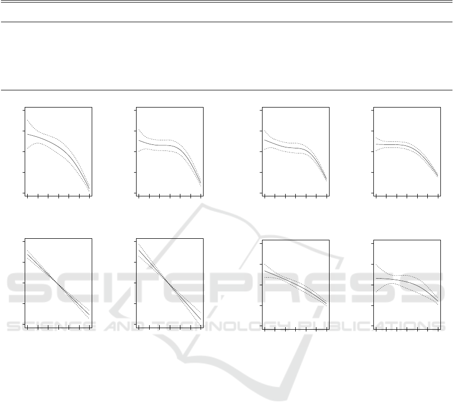
Table 2: Comparison of relativities of DR, separated by coverages. The relativities are obtained from modelling using GLM

and GAM and from empirical loss costs and premiums for the accident year 2009.

DR AB COL TPL

GLM GAM Loss Cost Premium GLM GAM Loss Cost Premium GLM GAM Loss Cost Premium

0 3.64 2.27 3.99 3.33 2.33 1.85 2.31 2.36 3.13 2.11 3.21 2.93

1 2.73 2.07 2.85 2.71 2.15 1.76 2.31 2.01 2.38 1.94 2.31 2.49

2 2.54 1.80 2.43 2.63 1.91 1.61 1.90 1.92 2.36 1.77 2.29 2.43

3 1.74 1.65 1.74 1.80 1.65 1.54 1.81 1.51 1.80 1.67 1.82 1.79

4 2.10 1.64 2.14 2.10 1.79 1.54 1.82 1.78 2.09 1.60 2.16 1.87

5 1.63 1.48 1.78 1.65 1.51 1.40 1.58 1.48 1.48 1.40 1.58 1.47

6 1.00 1.00 1.00 1.00 1.00 1.00 1.00 1.00 1.00 1.00 1.00 1.00

0 1 2 3 4 5 6

−1.0 −0.5 0.0 0.5 1.0

s(DR,2.26):factor(CLASS)CLASS1

(a) Class 1

0 1 2 3 4 5 6

−1.0 −0.5 0.0 0.5 1.0

s(DR,2.83):factor(CLASS)CLASS2

(b) Class 2

0 1 2 3 4 5 6

−1.0 −0.5 0.0 0.5 1.0

s(DR,1):factor(CLASS)CLASS3

0 1 2 3 4 5 6

−1.0 −0.5 0.0 0.5 1.0

s(DR,1):factor(CLASS)CLASS7

(d) Class 7

Figure 2: Functional patterns of DR for Class 1, Class 2,

Class 3 and Class 7 for AB coverage for 2009 accident year

data. The total risk exposures for these four classes account

for 92% of the vehicles.

We focus on the DR by major classes as the estimated

functional patterns are relatively stable. These four

major classes account for about 92% of risk expo-

sures. The deﬁnitions of these classes are given in

Table 1. The study based on the consideration of ma-

jor classes is more conclusive and may provide more

insights into DR. Thus, the results can serve as an im-

portant reference and be more beneﬁcial for auto in-

surance companies. From these results, we observe

that the variability of estimates for smaller DR are

higher than for the larger DR levels. This is generally

true for all cases and will be discussed later. The main

reason for this high variability is the smaller amounts

of risk exposure for lower levels of DR, which corre-

sponds to the drivers who have had accidents in recent

years. Also, from the obtained results, we observe

0 1 2 3 4 5 6

−1.0 −0.5 0.0 0.5 1.0

s(DR,2.9):factor(CLASS)CLASS1

(a) Class 1

0 1 2 3 4 5 6

−1.0 −0.5 0.0 0.5 1.0

s(DR,2.75):factor(CLASS)CLASS2

(b) Class 2

0 1 2 3 4 5 6

−1.0 −0.5 0.0 0.5 1.0

s(DR,1.47):factor(CLASS)CLASS3

0 1 2 3 4 5 6

−1.0 −0.5 0.0 0.5 1.0

s(DR,1.55):factor(CLASS)CLASS7

(d) Class 7

Figure 3: Functional patterns of DR for Class 1, Class 2,

Class 3 and Class 7 for COL coverage for 2009 accident

year loss data. The total risk exposures for these four classes

account for 92% of the vehicles.

that the functional patterns of DR are decreasing with

the increase of DR levels for all major Classes. How-

ever, the function patterns are different from Class to

Class, which implies the interaction of Class and DR.

These ﬁndings conﬁrm our expectations on the rela-

tionship between Class and DR, which is not inde-

pendent. Therefore, modelling loss cost or premium

using Class and DR one may has to further consider

such interaction, which may be extended to other fac-

tors if one has to consider.

The results obtained from COL and TPL are dis-

played in Figures 3 and 4, respectively. For these re-

sults, we observe that the functional patterns for Class

1 and 2 from the two considered coverages, COL and

TPL, do not appear to differ from those obtained from

the AB coverage. However, for Class 3 and Class 7,

Exploring Functional Patterns of Driving Records by Interacting with Major Classes and Territory Using Generalized Additive Models

275

0 1 2 3 4 5 6

−1.0 −0.5 0.0 0.5 1.0

s(DR,2.63):factor(CLASS)CLASS1

(a) Class 1

0 1 2 3 4 5 6

−1.0 −0.5 0.0 0.5 1.0

s(DR,2.48):factor(CLASS)CLASS2

(b) Class 2

0 1 2 3 4 5 6

−1.0 −0.5 0.0 0.5 1.0

s(DR,1):factor(CLASS)CLASS3

0 1 2 3 4 5 6

−1.0 −0.5 0.0 0.5 1.0

s(DR,1.77):factor(CLASS)CLASS7

(d) Class 7

Figure 4: Functional patterns of DR for Class 1, Class 2,

Class 3 and Class 7 for TPL coverage and 2009 accident

year loss data. The total risk exposures for these four classes

account for 92% of the vehicles.

especially for Class 7, the difference among the func-

tional patterns of DR for different coverages seems

to be large. This provides strong evidence of how the

DR functional pattern depends on or interacts with the

Class factor. This tells us that the assumption of inde-

pendence between DR and Class appears to be prob-

lematic when it comes to auto insurance policy pric-

ing. As the insurance pricing is done by coverage,

because of this interaction, it makes sense to model

the loss cost by estimating the relativity of DR, condi-

tioned on the Class factor. This may potentially elim-

inate the double penalty coming from the high-risk

groups, which is jointly determined by a set of highly

dependent factors.

To further investigate the functional patterns of

DR within a coverage but with a different level of

territory, i.e. Urban or Rural, we ﬁtted our data to

GAM with the DR conditioned on the Territory vari-

able. The obtained results are reported in Figure 5.

The results show that the functional pattern of DR for

coverages of AB and COL does not deviate much be-

tween Urban and Rural, but the patterns are signiﬁ-

cantly changed for TPL coverage. This may suggest

a low dependency between DR and Territory for AB

and COL coverage but a strong dependence between

them for TPL.

The above analysis demonstrates the potential in-

teraction between DR and other risk factors, i.e. Class

0 1 2 3 4 5 6

−1.0 −0.5 0.0 0.5 1.0

s(DR,3.6):factor(TERRITORY)0

(a) AB, Rural

0 1 2 3 4 5 6

−1.0 −0.5 0.0 0.5 1.0

s(DR,2.98):factor(TERRITORY)1

(b) AB, Urban

0 1 2 3 4 5 6

−1.0 −0.5 0.0 0.5 1.0

s(DR,3.51):factor(TERRITORY)0

0 1 2 3 4 5 6

−1.0 −0.5 0.0 0.5 1.0

s(DR,3.64):factor(TERRITORY)1

(d) COL,Urban

0 1 2 3 4 5 6

−1.0 −0.5 0.0 0.5 1.0

s(DR,3.75):factor(TERRITORY)0

(e) TPL, Rural

0 1 2 3 4 5 6

−1.0 −0.5 0.0 0.5 1.0

s(DR,2.38):factor(TERRITORY)1

(f) TPL,Urban

Figure 5: Comparison of functional DR patterns, separated

by coverage and territory (Urban and Rural) based on 2009

accident year loss data.

and Territory, used in rate regulation practice. Fur-

thermore, the decreasing patterns reasonably explain

how risk relativities will behave when derived using

the estimated function employing GAM. This may

suggest that a new risk measure of DR risk relativity

can be computed based on the functional pattern re-

sults obtained from GAMs, unlike the traditional ap-

proach of deriving risk relativity either empirically,

based on the loss cost, or by modelling based on

GLM. For the illustration purpose of using GAM,

we have computed the risk relativities and compared

these results with the relativities obtained from loss

cost, premium and GLM modelling. They are re-

ported in Table 2. For the relativity of DR at the whole

number scale, only the results obtained from GAM

meet the requirement of being monotonic. Also,

the results from GAM lower the relative difference

DATA 2023 - 12th International Conference on Data Science, Technology and Applications

276

0 1 2 3 4 5 6

1.0 1.5 2.0 2.5

Relativity

2009AB

2009COL

2009TPL

2010AB

2010COL

2010TPL

2011AB

2011COL

2011TPL

(a) Class 1

0 1 2 3 4 5 6

1.0 1.5 2.0 2.5

Relativity

2009AB

2009COL

2009TPL

2010AB

2010COL

2010TPL

2011AB

2011COL

2011TPL

(b) Class 2

0 1 2 3 4 5 6

1.0 1.5 2.0 2.5

Relativity

2009AB

2009COL

2009TPL

2010AB

2010COL

2010TPL

2011AB

2011COL

2011TPL

0 1 2 3 4 5 6

1.0 1.5 2.0 2.5 3.0

Relativity

2009AB

2009COL

2009TPL

2010AB

2010COL

2010TPL

2011AB

2011COL

2011TPL

(d) Class 7

Figure 6: DR relativities for Class 1, Class 2, Class 3

and Class 7 for different insurance coverage and accident

year combinations. The total risk exposures for these four

classes account for 92% of the vehicles.

among different levels, which may help address the

concern of having high relativity for the low level of

DR. The relativity associated with level zero obtained

from GAM is the smallest among all other cases.

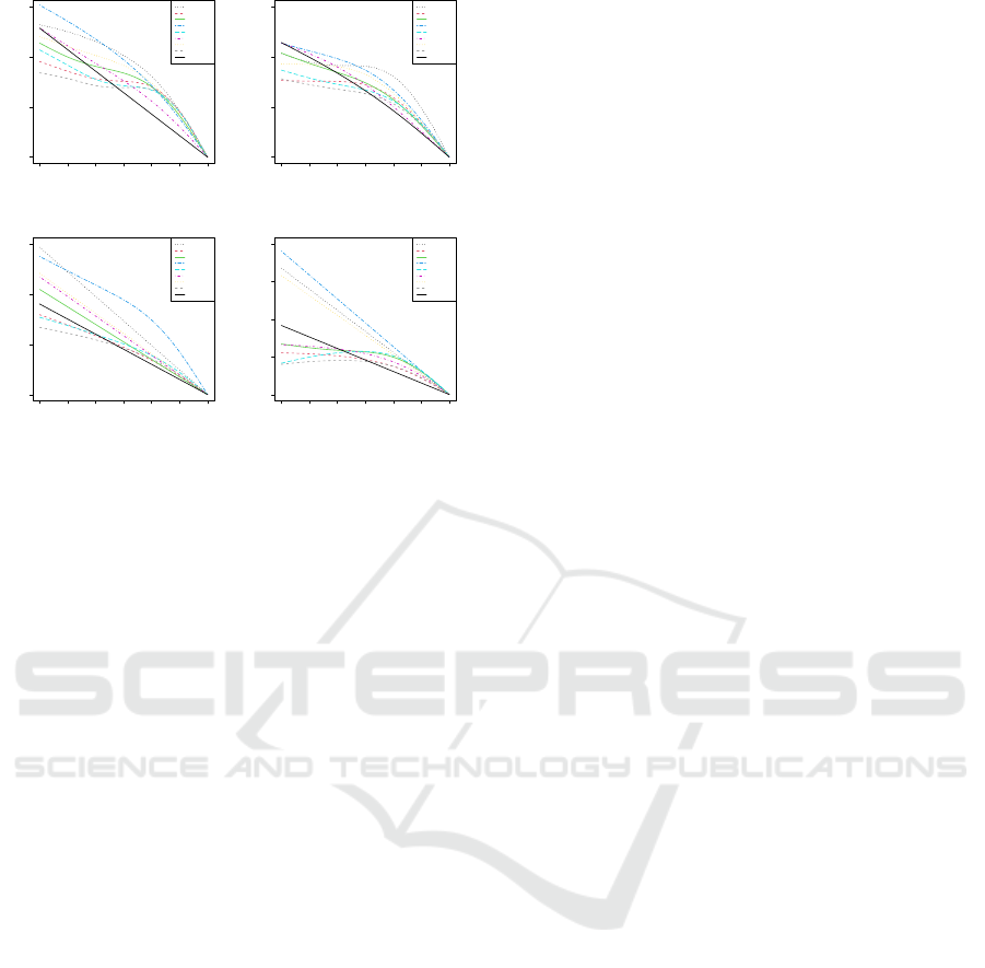
Finally, we study the risk relativity patterns of DR,

separated by different combinations of coverages and

accident years for each major class, to see how they

differ with a given class when the condition changes.

These relativity curves are presented in Figure 6. We

observe a considerable variation for Class 3 and Class

7, but functional variability for the curves with Class

1 and Class 2 are much smaller. Part of this vari-

ability may be due to the number of risk exposures,

as the total risk exposures for Class 1 and Class 2 is

much higher. The AB coverage has larger risk rela-

tivity spread for DR, especially for Class 7. Overall,

we can conclude that different combinations of acci-

dent and coverage for the different major classes have

different DR relativity patterns This may imply that

the analysis of loss cost and premium need to be done

by separating them by each combination. This also

indicates the dependency among all risk factors that

we considered, including coverages, accident years,

class, territory, and DR. Given the fact that low levels

of DR may be because of new drivers, it makes sense

to have relativity set to be lower than the ones from

Loss cost or other modelling methods based on the

loss cost. The fact that we constantly observe low val-

ues for DR relativities from GAM implies the sound-

ness of our proposed method to be an alternative ap-

proach for estimating DR relativities.

4 CONCLUDING REMARKS

Studying the safe driver index and other risk factors

in auto insurance rate regulation has been of an on-

going interest. Research on this topic has shown the

need for the development and application of advanced

statistical techniques to obtain an improved insights

into loss and premium data. By modelling the inter-

action between DR and Class using loss cost and pre-

mium data, while including other explanatory vari-

ables such as territory, we can uncover the different

patterns when looking at DR alone could not uncover

them. This work focused on using GAM to model

the functional relationship between DR and the re-

sponse variable with the inclusion of interaction fac-

tors, Class and Territory. We used GAMS to model

non-linear relationships captured by additive compo-

nents of splines. We further proposed to use the ob-

tained smooth functions of DR to derive its risk rela-

tivity.

Despite GAM requiring more computational

power due to its higher complexity than linear or gen-

eralized linear models, GAMs balance linear models

and black box machine learning models in terms of

interpretability and ﬂexibility of the model used. Ex-

amining how speciﬁc risk factors predict the outcome

of risk relativities can give a better understanding of

what factors auto insurance companies ﬁnd signiﬁ-

cant. Extension of this work could investigate the

relationships of other risk factors that inﬂuence auto

insurance pricing, such as the interaction of gender

and age with driving records using GAMs. The ﬂex-

ibility of GAM models can help uncover hidden pat-

terns between risk factors and risk relativity. The pro-

posed method can also be applied to other types of

economic and business data where the functional re-

lationship between independent variables and the de-

pendent variable need to be captured, and functional-

ity of some independent variables need to be embed-

ded.

ACKNOWLEDGEMENT

ATL acknowledges partial support from Natural Sci-

ences and Engineering Research Council of Canada.

REFERENCES

Abraham, K. S. (1985). Efﬁciency and fairness in insurance

risk classiﬁcation. Virginia Law Review, pages 403–

451.

Boucher, J.-P., C

e, S., and Guillen, M. (2017). Exposure

Exploring Functional Patterns of Driving Records by Interacting with Major Classes and Territory Using Generalized Additive Models

277

as duration and distance in telematics motor insurance

using generalized additive models. Risks, 5(4):54.

Brown, R. L., Charters, D., Gunz, S., and Haddow, N.

(2004). Age as an insurance rate class variable.

Burka, D., Kov

acs, L., and Szepesv

ary, L. (2021). Mod-

elling mtpl insurance claim events: Can machine

learning methods overperform the traditional glm ap-

proach? Hungarian Statistical Review, 4(2):34–69.

Denuit, M., Charpentier, A., and Truﬁn, J. (2021). Autocal-

ibration and tweedie-dominance for insurance pricing

with machine learning. Insurance: Mathematics and

Economics, 101:485–497.

Frezal, S. and Barry, L. (2020). Fairness in uncertainty:

Some limits and misinterpretations of actuarial fair-

ness. Journal of Business Ethics, 167:127–136.

Hastie, T. J. (2017). Generalized additive models. In Statis-

tical models in S, pages 249–307. Routledge.

Huang, Y. and Meng, S. (2019). Automobile insurance clas-

siﬁcation ratemaking based on telematics driving data.

Decision Support Systems, 127:113156.

Landes, X. (2015). How fair is actuarial fairness? Journal

of Business Ethics, 128:519–533.

Meng, S., Wang, H., Shi, Y., and Gao, G. (2022). Improv-

ing automobile insurance claims frequency prediction

with telematics car driving data. ASTIN Bulletin: The

Journal of the IAA, 52(2):363–391.

Meyers, G. and Van Hoyweghen, I. (2018). Enacting ac-

tuarial fairness in insurance: From fair discrimina-

tion to behaviour-based fairness. Science as Culture,

27(4):413–438.

Ohlsson, E. and Johansson, B. (2010). Non-life insurance

pricing with generalized linear models, volume 174.

Springer.

Rolison, J. J., Regev, S., Moutari, S., and Feeney, A. (2018).

What are the factors that contribute to road accidents?

an assessment of law enforcement views, ordinary

drivers’ opinions, and road accident records. Accident

Analysis & Prevention, 115:11–24.

Wood, S. N. (2006). Generalized additive models: an intro-

duction with R. chapman and hall/CRC.

Xie, S. (2021). Improving explainability of major risk fac-

tors in artiﬁcial neural networks for auto insurance

rate regulation. Risks, 9(7):126.

Xie, S. and Lawniczak, A. T. (2018). Estimating major risk

factor relativities in rate ﬁlings using generalized lin-

ear models. International Journal of Financial Stud-

ies, 6(4):84.

DATA 2023 - 12th International Conference on Data Science, Technology and Applications

278