Simulation of Steady and Transient 3D Flows via Physics-Informed Deep

Learning

Philipp Moser

, Wolfgang Fenz

, Stefan Thumfart

, Isabell Ganitzer

and Michael Giretzlehner

Research Department Medical Informatics, RISC Software GmbH, Softwarepark 32a, 4232 Hagenberg, Austria

Keywords:

Physics-Informed Neural Networks, Fluids, Navier-Stokes, Deep Learning.

Abstract:

Physics-Informed deep learning methods are attracting increased attention for modeling physical systems due

to their mesh-free approach, their straightforward handling of forward and inverse problems, and the possi-

bility to seamlessly include measurement data. Today, most learning-based ﬂow modeling reports rely on

the representational power of fully-connected neural networks, although many different architectures have

been introduced into deep learning, each with speciﬁc beneﬁts for certain applications. In this paper, we suc-

cessfully demonstrate the application of physics-informed neural networks for modeling steady and transient

ﬂows through 3D geometries. Our work serves as a practical guideline for machine learning practitioners by

comparing several popular network architectures in terms of accuracy and computational costs. The steady

ﬂow results were in good agreement with ﬁnite element-based simulations, while the transient ﬂows proved

more challenging for the continuous-time PINN approaches. Overall, our ﬁndings suggest that standard fully-

connected neural networks offer an efﬁcient balance between training time and accuracy. Although not readily

supported by statistical/practical signiﬁcance, we could identify a few more complex architectures, namely

Fourier networks and Deep Galerkin Methods, as attractive options for accurate ﬂow modeling.

1 INTRODUCTION

In recent years, the remarkable advances of deep

learning (DL) in various domains (e.g., computer vi-

sion and natural language processing) have inspired

vibrant research on applying DL to obtain solutions

for physical models, which, in general, has become

an integral part of modern science. While physics-

based DL comprises a variety of conceptually dif-

ferent approaches (Karniadakis et al., 2021), we fo-

cus on physics-informed DL that encodes physical in-

formation (typically expressed as partial differential

equations (PDEs) with suitable initial/boundary con-

ditions) into the loss function of a neural network,

hence, constraining the network’s trainable param-

eters. An overview of Raissi’s general framework

of physics-informed neural networks (PINNs) (Raissi

et al., 2019) is given in Section 1.1. Compared to con-

https://orcid.org/0000-0002-9717-6197

https://orcid.org/0000-0002-6143-3024

https://orcid.org/0000-0001-9838-3641

https://orcid.org/0000-0003-3600-0857

https://orcid.org/0000-0003-1620-1002

ventional computational ﬂuid dynamics (CFD) meth-

ods, PINNs operate without the need to mesh the sim-

ulation geometry and can easily handle forward sim-

ulations (predicting state or temporal evolution) or in-

verse problems (e.g., obtaining a parametrization for

a physical system from observations).

Fluid mechanics is among the most active research

topics due to (a) the complex underlying Navier-

Stokes equations, (b) the lack of general analytic

solutions and (c) the widespread applications (e.g.,

biomedical engineering, geophysics, aerospace). Se-

lected PINN applications include the prediction of

near-wall blood ﬂow from sparse data (Arzani et al.,

2021), direct turbulence modeling (Jin et al., 2021),

solving the Reynolds-averaged Navier–Stokes equa-

tions (Eivazi et al., 2022), tackling ill-posed inverse

ﬂuid-mechanics problems (Raissi et al., 2020), or

mixed-variable PINN schemes for 2D ﬂows (Rao

et al., 2020).

Deep learning is a fast-evolving ﬁeld of research

where many network architectures and add-ons (e.g.,

Fourier encoding layers, adaptive activation func-

tions, skip connections) have been proposed (Choud-

hary et al., 2022; Markidis, 2021). Despite the broad

Moser, P., Fenz, W., Thumfart, S., Ganitzer, I. and Giretzlehner, M.

Simulation of Steady and Transient 3D Flows via Physics-Informed Deep Learning.

DOI: 10.5220/0012078600003546

In Proceedings of the 13th Inter national Conference on Simulation and Modeling Methodologies, Technologies and Applications (SIMULTECH 2023), pages 243-250

ISBN: 978-989-758-668-2; ISSN: 2184-2841

 2023 by SCITEPRESS – Science and Technology Publications, Lda. Under CC license (CC BY-NC-ND 4.0)

243

architectural variety, to date the majority of PINN-

based ﬂow simulations have employed simple fully-

connected neural networks (FCNNs) (Jin et al., 2021;

Eivazi et al., 2022; Oldenburg et al., 2022; Arzani

et al., 2021; Amalinadhi et al., 2022). Only few

publications report the use of more complex network

architectures, such as convolutional neural networks

(CNNs) (Ma et al., 2022; Eichinger et al., 2021;

Guo et al., 2016; Gao et al., 2021) or Deep Galerkin

Methods (DGMs) (Matsumoto, 2021; Li et al., 2022).

While this is related to the early development phase of

PINNs and the initial focus on feasibility and proof-

of-concept (Cuomo et al., 2022; Karniadakis et al.,

2021), the increasing interest in PINNs motivates the

integration and evaluation of recent DL developments

that have shown promising results in other applica-

tions. Comparing results across publications is of-

ten difﬁcult because of signiﬁcant variations in sim-

ulation domains (2D or 3D), ﬂuid characteristics and

evaluation metrics.

In this paper, we ﬁll this gap and provide the

ﬁrst comprehensive comparison of several popular

network architectures for modeling steady and tran-

sient ﬂows in 3D geometries. Besides standard FC-

NNs, we evaluate the computational costs and accu-

racy of (in total) seven different architectures using

ﬁnite element-based CFD models as references. Our

comparative analysis intends to highlight the potential

but also the challenges of current PINN architectures

for modeling ﬂuid dynamics.

1.1 Principles of Physics-Informed

Neural Networks

In general, a physical system is governed by a set

of PDEs that describe the variation of some physical

quantity u (e.g., velocity in the case of ﬂuid dynam-

ics) at points x ∈ Ω (i.e., points within a geometry

Ω). Most often, these PDEs are accompanied by (a)

boundary conditions B which specify the values of u

at points x on the boundary ∂Ω and (b) initial condi-

tions I which deﬁne the values of u at t = 0.

Raissi et al. introduced PINNs (Raissi et al.,

2019), which aim at approximating the complex (and

nonlinear) solution function u via a deep neural net-

work. Physics information (given by the underlying

PDE), boundary constraints, initial conditions as well

as sparse measurement data (if available) are inte-

grated into the loss function of a neural network:

tot

= L

PDE

+ L

data

. (1)

PDE

evaluates (via the two-norm

∥

) the PDE’s

residual on randomly sampled points within the ge-

Neural network Auto-differentiation Loss function

Adam optimizer

Update NN's

weights & biases

Total loss function

physics-informed loss

BC-related loss

IC-related loss

data-informed loss

∂

(n)

∂

Figure 1: Schematic of a PINN. The physical quantities of

interest are (u, v, w, p) and the spatio-temporal coordinates

are (x, y, z, t). σ is the activation function.

ometry Ω

PDE



N (x, u,t)



Ω

, (2)

with N being the PDE’s nonlinear differential oper-

ator. L

is sampled on points on the boundary ∂Ω

where boundary conditions B are known:

∥

B(x, u,t)

∥

∂Ω

, (3)

while L

is calculated from initial conditions I with

sampling points at t = 0:

∥

I (x, u,t = 0)

∥

. (4)

The data loss term L

data

is evaluated on discrete

points Γ where additional measurement data D is

available:

data

∥

u − D

∥

. (5)

The PINN training process is depicted in Figure 1.

A neural network generates estimates for u on a set

of randomly sampled spatio-temporal points (x, y, z,t).

Using auto-differentiation, all necessary derivatives

are generated and allow for the calculation of the

PDE-related (physics-informed) loss term L

PDE

. The

total loss function L

tot

is constructed by adding all

four loss terms in Eq. 1. While training the network,

the optimal set of weights and biases of the neural

network is being sought, for which the total loss func-

tion is minimized and the resulting estimates for u ap-

proach the true solution.

2 METHODS

2.1 Simulation Model, Geometries and

Ground Truth

The ﬂow of incompressible Newtonian ﬂuids is de-

scribed by the Navier-Stokes and continuity equa-

tions:



∂u

∂t

+ (u · ∇)u



− µ∇

u + ∇p = 0, (6)

∇ · u = 0. (7)

SIMULTECH 2023 - 13th International Conference on Simulation and Modeling Methodologies, Technologies and Applications

244

Cylinder

(b)

(a)

Stenosed Cylinder

(c)

0.2

v [m/s]

0.0

0.0 0.5 1.0 1.5 2.0

t [s]

0.2

0.4

0.6

0.8

1.0

f(t)

Figure 2: (a) The parabolic inlet velocity proﬁle, (b) the

time-varying inﬂow function f (t), (c) the two studied ge-

ometries. The inﬂow is indicated by a red arrow.

u = u(x, t) = [u(x,t), v(x,t), w(x,t)]

⊺

denotes the ve-

locity vector and p = p(x,t) is the pressure ﬁeld. The

inﬂow was set perpendicular to the inlet plane with a

parabolic velocity proﬁle:

inlet

(r) = u

max



1 −



, (8)

with r being the radial distance from the inlet cen-

ter and R being the radius of a cylindrical inlet. The

central peak velocity u

max

was set to 0.2 m/s, see Fig-

ure 2a. A pulsatile ﬂow was generated by a tempo-

rally varying function f (t) using a Gaussian-shaped

pulse with a duration of 1.0 s, see Figure 2b. The en-

tire time-varying inﬂow proﬁle u

inlet

(r, t) is obtained

by multiplying u

inlet

(r) (from Eq. 8) and f (t) (de-

picted in Figure 2b). The total simulation time was

set to 2.0 s.

We modeled two cylindrical geometries (Fig-

ure 2c) that frequently appear in various engineering

domains (e.g., modeling healthy and diseased arteries

in computational hemodynamics). Speciﬁcally, the

ﬁrst system was the laminar ﬂow of a ﬂuid (density

ρ = 1233 kg/m

, dynamic viscosity µ = 0.20393 Pa·s,

Reynolds number Re = 1209) through a regular cylin-

der (radius: 0.5 m, length: 5 m). The second geome-

try was a cylinder with a stenosis created by a sphere

of radius of 0.5 m centered on its surface 1.25 m from

the inlet. The ﬂuid parameters (ρ = 616.5 kg/m

µ = 0.40786 Pa·s, Re = 302) differed from the ﬁrst

system to showcase PINN’s ability to handle various

regimes of laminar ﬂuid properties. We employed the

following boundary conditions: no-slip conditions on

the geometry walls (u, v, w = 0) and the pressure set

to zero at the outlet (p = 0).

Ground truth (reference) distributions of velocity

and pressure were generated via ﬁnite-element-based

simulations using the framework MODSIM, an in-

house CFD software suite (Fenz et al., 2010; Fenz

et al., 2016; Gmeiner et al., 2018). Both CFD geome-

tries had around 600k mesh points. All simulations

(i.e., PINN and CFD modeling) were performed on a

workstation with an Intel i9-11900 (CPU), NVIDIA

GeForce RTX 3080 Ti (GPU) and 64 GB RAM.

2.2 Network Architectures

We implemented all PINN architectures within

NVIDIA’s Modulus framework v22.03 (Hennigh

et al., 2021; NVIDIA, 2022). For comparison pur-

poses, the same network size (6 layers with 256 neu-

rons each), swish activation functions (β=1), expo-

nentially decaying learning rates (initial learning rate:

0.0005, decay rate: 0.97, decay steps: 20005) and

Adam optimizers were used across all network archi-

tectures. In the following, the seven studied architec-

tures are brieﬂy summarized. More information can

be obtained in the referenced original publications.

2.2.1 Fully Connected Neural Networks

In the standard version, all neurons of one layer are

connected to each neuron in the next layer. The output

of an n-layer FCNN u

net

(x;θ) reads

net

(x;θ) = W

{φ

n−1

◦φ

n−2

◦ ··· ◦ φ

}(x)+b

, (9)

) = σ(W

+ b

), (10)

where φ

is the i

layer, W

and b

are the weights

and biases of the i

layer. θ refers to the trainable

parameters {W

, b

}

i=1

. Throughout the architecture

descriptions, σ is the activation function and the vec-

tor notation x includes all spatial and temporal coor-

dinates x = (x, y, z;t).

The second architecture (termed FCNNaa) is a

variation of simple FCNNs and features adaptive acti-

vation functions as suggested by Jagtap et al. (Jagtap

et al., 2020). A global, trainable, multiplicative pa-

rameter α is added to the activation functions and the

layer of the FCNN, hence, becomes

) = σ(α · (W

+ b

)). (11)

The third architecture (termed FCNNskip) is a further

variation of FCNNs which includes skip connections

every two hidden layers. Originally introduced into

deep learning for addressing the vanishing gradient

problem (He et al., 2016), skip connections feed the

output of one layer as the input to the next layers (in-

stead of only the subsequent layer).

2.2.2 Fourier Networks

The fourth architecture (termed FN) is a Fourier net-

work which tries to reduce spectral biases (Rahaman

et al., 2019; Tancik et al., 2020; Mildenhall et al.,

2020). A FCNN architecture is modiﬁed by adding

an initial Fourier encoding layer φ

that includes a

trainable frequency matrix m

net

(x;θ) = W

{φ

n−1

◦ φ

n−2

◦ ···◦ φ

◦ φ

}(x)+b

(12)

Simulation of Steady and Transient 3D Flows via Physics-Informed Deep Learning

245

= [sin (2πm

· x); cos (2πm

· x)]

. (13)

The ﬁfth architecture (termed modFN) is a mod-

iﬁed Fourier network. It uses two additional layers

that transform the Fourier features to a learned feature

space and transfer the information ﬂow to the other

hidden layers via Hadamard multiplications (denoted

by ⊙) (Wang et al., 2021). Here, the i

layer reads:

) = (1 − σ(W

+ b

)) ⊙ σ(W

+ b

) +

σ(W

+ b

) ⊙ σ(W

+ b

) for i > 1.

(14)

The additional trainable parameters

, b

, W

, b

} belong to the two added

transformation layers.

2.2.3 Multiplicative Filter Network (MFN)

The sixth architecture is a Fourier MFN which gen-

erates representational power through repeated multi-

plications of sinusoidal wavelet functions f(x, ξ

) ap-

plied to the input (Fathony et al., 2021):

f(x, ξ

) = sin (ω

x + φ

) with ξ

= (ω

, φ

= f(x, ξ

i+1

= σ(W

+ b

) ⊙ f (x, ξ

i+1

), ∀i ∈ {1, ..., n − 1},

net

(x;θ) = W

+ b

(15)

2.2.4 Deep Galerkin Method (DGM)

The DGM approach as proposed by Sirignano and

Spiliopoulos is the seventh architecture. Inspired

by the well-established Galerkin method, the DGM

replaces the linear combination of basis functions

to approximate the PDE’s solution by a deep neu-

ral network. The architecture is rather complex and

has some similarities to Long Short-Term Memory

(LSTM) networks. For the explicit network struc-

ture, we refer to the original publication (Sirignano

and Spiliopoulos, 2018).

2.3 Evaluation Metrics

To compare the accuracy of the PINN results against

CFD simulations, we calculated mean absolute er-

rors (MAE) and standard deviations of absolute er-

rors (STD of AE) of the physical quantities of inter-

est (i.e., absolute velocity and pressure): The PINNs

were evaluated at the CFD mesh points and the error

metrics were calculated based on the absolute differ-

ences of the PINN and CFD solutions.

Regarding statistical analysis, we calculated Co-

hen’s effect size d (Lakens, 2013) to assess the prac-

tical signiﬁcance of the differences in MAEs between

the best-performing architecture and all others.

3 RESULTS

3.1 Steady Flow

For the steady ﬂow simulations, the MAEs and STDs

of AE for all used PINN architectures are summarized

in Table 1. In the regular cylinder, the lowest MAE in

absolute velocity was obtained for the FN architec-

ture. However, all MAEs were close to each other

with overlapping 95% conﬁdence intervals and effect

sizes d below 0.2 suggesting practically insigniﬁcant

differences in accuracy among the architectures.

In the stenosed cylinder, the MAEs in absolute ve-

locity had a broader range and the values were gen-

erally higher (which was expected due to the higher

geometrical complexity), with modFN performing

far worse than all other architectures. The DGM

performed best, however, the effect sizes between

DGM and the other architectures were small indicat-

ing rather low practical importance.

In both cylinder geometries, FCNNskip per-

formed best in terms of pressure MAE, while modFN

performed worst with effect sizes d > 0.9 suggesting

considerably worse results.

Figure 3 depicts the predicted (i.e., learned) distri-

butions of the absolute velocity and pressure as well

as their absolute deviations from CFD references. At

the inlet of the regular cylinder, a mean pressure of

3.38 Pa was obtained with FCNNskip, while the an-

alytic values would be 3.26 Pa (calculated via the

Hagen–Poiseuille equation which describes the ﬂow

pressure drop in a cylindrical pipe).

Stenosed Cylinder (DGM)

Absolute Errors

Cylinder (FN)

Figure 3: Steady ﬂow simulations: The predicted absolute

velocity and pressure distributions (ﬁrst row), as well as

their absolute errors (AEs) (second row). The shown ar-

chitectures were chosen based on the best absolute velocity

estimates.

The training times for one epoch are also compiled

in Table 1 and show signiﬁcant variations: The DGM,

for example, required about a factor 3.9 more time to

train than a standard FCNN. In absolute numbers, the

FCNN training (with 350 epochs) of the steady ﬂow

system took around 9.6 hours on our hardware.

SIMULTECH 2023 - 13th International Conference on Simulation and Modeling Methodologies, Technologies and Applications

246

Table 1: Steady ﬂow simulations: Errors metrics for the various PINN architectures. Note: The velocity errors are given in

mm/s. The percentage values in the last column are relative to the FCNN architecture. Bold numbers indicate the best results.

MAE and STD of AEs Training time

Cylinder Stenosed Cylinder per epoch [s]

Abs Vel [mm/s] Pressure [Pa] Abs Vel [mm/s] Pressure [Pa]

FCNN 0.838±0.405 0.075±0.060 1.024±0.899 0.066±0.075 99 (100%)

FCNNaa 0.837±0.406 0.073±0.062 0.990±0.823 0.054±0.075 113 (114%)

FCNNskip 0.819±0.412 0.068±0.058 1.201±1.107 0.052±0.054 101 (102%)

FN 0.801±0.387 0.076±0.061 1.188±1.051 0.055±0.079 100 (101%)

modFN 0.813±0.486 0.342±0.194 25.514±24.163 1.696±1.226 178 (178%)

MFN 0.838±0.383 0.105±0.051 0.918±0.840 0.056±0.072 103 (104%)

DGM 0.843±0.387 0.076±0.046 0.819±0.693 0.053±0.075 384 (388%)

3.2 Transient Flow

For the transient ﬂow simulations, we calculated

MAEs every 0.05 seconds and visualize their tempo-

ral evolution in Figure 4. Overall, the lowest MAEs

were recorded for the FCNN, FN and DGM archi-

tectures, while MFN and modFN performed signiﬁ-

cantly worse. MAEs of absolute velocity were gen-

erally lower than for the pressure estimates. For

all architectures, the highest MAEs occured between

t = 0.5 s and t = 1.0 s (which includes the peak of

the Gaussian inﬂow proﬁle and the region of fastest

change in inﬂow). Still, differences regarding the

shape of the temporal MAE curves were observed

among architectures.

The predicted absolute velocity and pressure dis-

tributions at three speciﬁc points in time are visual-

ized in Figure 5. The time point t = 1.00 s corre-

sponds to the half maximum on the right side of the

inﬂow proﬁle (see Figure 4). Noticeable deviations

were observed throughout the pressure estimates with

relative AEs (i.e., AEs normalized by the absolute

CFD reference) being highest in the ﬂat part of the

inﬂow proﬁle.

4 DISCUSSION

An integral part of an effective and efﬁcient learn-

ing framework involves the design and selection of

the network architecture. The training process (i.e.,

the convergence and accuracy of the learned solution)

can be positively inﬂuenced when a domain-intrinsic

property is reﬂected within the architecture. CNNs,

for example, unfold their strength in image-related

tasks as convolution operators reﬂect the translational

invariance of images. Unfortunately, no such intrinsic

symmetry was identiﬁed for PINN-based ﬂuid mod-

eling, which results in PINNs mostly relying on the

representational power of FCNNs. Also, our PINN

approach of randomly sampling points within (irreg-

ular) geometries prohibited the use of convolutional

architectures as these rely on structured grids (as is

the case for images). Future research in geometric

DL may provide ways of leveraging convolutions in

non-Euclidean spaces.

In this paper, we have not only successfully

demonstrated the modeling of steady and transient

3D ﬂows, but also investigated the performance of

various network architectures. To our knowledge a

comparable evaluation has only been published for

steady ﬂows so far (Moser et al., 2023), while tran-

sient ﬂows have not been investigated before. Over-

all, the learned solutions were in good agreement with

CFD references, especially for the steady ﬂows, while

the increased complexity of time-dependent systems

was obviously more challenging. The higher errors

of the transient pressure estimates can be attributed to

the networks struggling with multi-scale issues: The

pressure distributions ranged over 4000 Pa, resulting

in single-digit pressures being challenging to resolve.

Although beneﬁts (improved convergence and so-

lution accuracy) were reported for adaptive activation

functions (Jagtap et al., 2020), we did not observe dis-

tinct improvements compared to standard FCNNs that

would favor their usage, especially when taking into

account their higher computational costs. Our ﬁnd-

ings regarding FCNNskip were mixed since the best

pressure estimates were obtained with FCNNskip in

the steady ﬂow simulations, while the transient ﬂow

results lagged behind standard FCNNs at equally fast

training times. FNs and DGMs achieved overall good

results and could match/outperform FCNNs. We ob-

tained good results with MFNs for the steady ﬂow

simulations, but their multiplicative way of generat-

ing representational power was insufﬁcient for time-

dependent problems.

Signiﬁcant differences in computational costs

were observed among the studied network architec-

tures which are mainly dominated by the complex-

ity of the architecture (e.g., the number of trainable

Simulation of Steady and Transient 3D Flows via Physics-Informed Deep Learning

247

Figure 4: Transient ﬂow simulations: The MAEs of the predicted absolute velocity (given in mm/s) and pressure distributions.

Note: The dashed line is the Gaussian inﬂow proﬁle which serves only as temporal guidance and is not the ”target curve”.

parameters). The DGM, for example, uses roughly

eight times more parameters in each hidden layer than

a usual dense layer (Al-Aradi et al., 2022), which sig-

niﬁcantly increases memory consumption and train-

ing time. While the presented relative computational

times are generally applicable, the absolute training

times are highly dependent on the available resources.

Multi-GPU systems and efﬁcient handling of tensor

operations (e.g., NVIDIA’s TensorFloat-32) should

further accelerate the training.

Overall, our ﬁndings suggest that FCNNs (with or

without skip connections) are an efﬁcient (accuracy

per unit training time) starting point due to their fast

training and consistent mid-to-high-tier results. Keep-

ing in mind that differences in accuracy were not al-

ways supported by (practical) signiﬁcance, we could

still identify a trend that some more complex archi-

tectures, such as FNs or DGMs, might be attractive

options for complex ﬂow modeling.

In this paper, we employed the continuous time

approach for transient systems, i.e., the time is treated

similar to the other continuous, spatial variables.

While this is a straightforward extension of steady-

state modeling, one potential limitation is the high

amount of sampling points needed to enforce physics

constraints in the entire spatio-temporal domain, es-

pecially in higher dimensions, longer simulation time

spans and complex geometries. Other publications

have discussed improvements of discrete time models

(Runge-Kutta time-stepping schemes) (Raissi et al.,

2019) or alternative network architectures (e.g., Re-

current Neural Networks) for modeling (longer) tem-

poral dynamics (Wu et al., 2022).

In this paper, we restrict our simulations to lam-

inar ﬂows at low Reynolds numbers. However, the

PINN approach could readily be applied to turbu-

lent ﬂows with higher Reynolds numbers since turbu-

lences are inherently described by the Navier-Stokes

equation. To adequately resolve (chaotic) changes in

pressure and ﬂow velocities, (a) signiﬁcantly more

sampling points would be necessary during train-

ing (increased memory consumption and computation

times) or (b) alternative approaches such as super-

resolution (Jiang et al., 2020) could be applied.

Future research may investigate the inﬂuence of

network hyperparameters, such as network sizes and

activation functions. Also, the generalizability of

a trained network to changes in ﬂuid parameters or

geometry may involve ﬁne-tuning/transfer-learning

techniques, which remains an effort for future stud-

ies.

5 CONCLUSIONS

In this paper, we addressed the practically relevant

question which network architectures in the rapidly

evolving ﬁeld of deep learning provide good learning

SIMULTECH 2023 - 13th International Conference on Simulation and Modeling Methodologies, Technologies and Applications

248

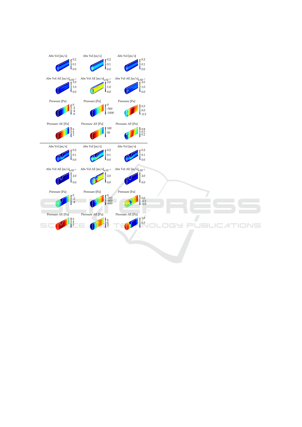
Stenosed Cylinder (DGM)

Cylinder (FCNN)

t= 0.0 s t= 1.0 s

t= 2.0 s

Figure 5: Transient ﬂow simulations: The predicted abso-

lute velocity and pressure distributions, as well as their ab-

solute errors are shown for three distinct points in time. The

network architectures with the best velocity estimates are

shown. Note: The absolute velocity and their error distribu-

tions share a common color range.

abilities to model the dynamics of ﬂuids in 3D ge-

ometries. While steady ﬂows could be modeled with

high accuracy, the transient ﬂows were more chal-

lenging to resolve with our continuous-time PINNs.

We conclude that while the investigated PINN imple-

mentations were in general capable of modeling the

complex behavior of ﬂuids, future architectures that

intrinsically reﬂect some underlying physical prop-

erty/symmetry and adequately handle multi-scale be-

haviors have the potential to outperform current ap-

proaches.

ACKNOWLEDGEMENTS

This project is ﬁnanced by research subsidies granted

by the government of Upper Austria within the re-

search projects MIMAS.ai, MEDUSA (FFG grant no.

872604) and ARES (FFG grant no. 892166). RISC

Software GmbH is Member of UAR (Upper Austrian

Research) Innovation Network.

REFERENCES

Al-Aradi, A., Correia, A., Jardim, G., de Freitas Naiff,

D., and Saporito, Y. (2022). Extensions of the deep

galerkin method. Applied Mathematics and Computa-

tion, 430:127287.

Amalinadhi, C., Palar, P. S., Stevenson, R., and Zuhal, L.

(2022). On physics-informed deep learning for solv-

ing navier-stokes equations. In AIAA SCITECH 2022

Forum.

Arzani, A., Wang, J.-X., and D’Souza, R. M. (2021). Un-

covering near-wall blood ﬂow from sparse data with

physics-informed neural networks. Physics of Fluids,

33(7):071905.

Choudhary, K., DeCost, B., Chen, C., Jain, A., Tavazza, F.,

Cohn, R., Park, C. W., Choudhary, A., Agrawal, A.,

Billinge, S. J. L., Holm, E., Ong, S. P., and Wolver-

ton, C. (2022). Recent advances and applications of

deep learning methods in materials science. npj Com-

putational Materials, 8(1):1–26.

Cuomo, S., Di Cola, V. S., Giampaolo, F., Rozza, G.,

Raissi, M., and Piccialli, F. (2022). Scientiﬁc machine

learning through physics–informed neural networks:

Where we are and what’s next. Journal of Scientiﬁc

Computing, 92(3):88.

Eichinger, M., Heinlein, A., and Klawonn, A. (2021). Sta-

tionary ﬂow predictions using convolutional neural

networks. Lecture Notes in Computational Science

and Engineering, Numerical Mathematics and Ad-

vanced Applications ENUMATH 2019, pages 541–

549.

Eivazi, H., Tahani, M., Schlatter, P., and Vinuesa, R.

(2022). Physics-informed neural networks for solving

reynolds-averaged navier–stokes equations. Physics

of Fluids, 34(7):075117.

Fathony, R., Sahu, A. K., Willmott, D., and Kolter, J. Z.

(2021). Multiplicative ﬁlter networks. In International

Conference on Learning Representations.

Fenz, W., Dirnberger, J., and Georgiev, I. (2016).

Blood ﬂow simulations with application to cerebral

aneurysms. In Proceedings of the Modeling and Simu-

lation in Medicine Symposium, pages 3:1–3:8. Society

for Computer Simulation International.

Fenz, W., Dirnberger, J., Watzl, C., and Krieger, M. (2010).

Parallel simulation and visualization of blood ﬂow in

intracranial aneurysms. In 11th IEEE/ACM Interna-

tional Conference on Grid Computing, pages 153–

160. ISSN: 2152-1093.

Simulation of Steady and Transient 3D Flows via Physics-Informed Deep Learning

249

Gao, H., Sun, L., and Wang, J.-X. (2021). Phy-

GeoNet: Physics-informed geometry-adaptive convo-

lutional neural networks for solving parameterized

steady-state PDEs on irregular domain. Journal of

Computational Physics, 428:110079.

Gmeiner, M., Dirnberger, J., Fenz, W., Gollwitzer, M.,

Wurm, G., Trenkler, J., and Gruber, A. (2018). Virtual

cerebral aneurysm clipping with real-time haptic force

feedback in neurosurgical education. World Neuro-

surgery, 112:e313–e323.

Guo, X., Li, W., and Iorio, F. (2016). Convolutional neural

networks for steady ﬂow approximation. In Proceed-

ings of the 22nd ACM SIGKDD International Con-

ference on Knowledge Discovery and Data Mining,

KDD ’16, pages 481–490.

He, K., Zhang, X., Ren, S., and Sun, J. (2016). Deep resid-

ual learning for image recognition. 2016 IEEE Con-

ference on Computer Vision and Pattern Recognition

(CVPR), pages 770–778.

Hennigh, O., Narasimhan, S., Nabian, M. A., Subrama-

niam, A., Tangsali, K., Fang, Z., Rietmann, M.,

Byeon, W., and Choudhry, S. (2021). NVIDIA Sim-

Net™: an AI-accelerated multi-physics simulation

framework. In Computational Science – ICCS 2021:

21st International Conference, Krakow, Poland, Pro-

ceedings, Part V, page 447–461. Springer-Verlag.

Jagtap, A. D., Kawaguchi, K., and Karniadakis, G. E.

(2020). Adaptive activation functions accelerate con-

vergence in deep and physics-informed neural net-

works. Journal of Computational Physics, 404.

Jiang, C. M., Esmaeilzadeh, S., Azizzadenesheli, K.,

Kashinath, K., Mustafa, M., Tchelepi, H. A., Marcus,

P., Prabhat, M., and Anandkumar, A. (2020). MESH-

FREEFLOWNET: A physics-constrained deep con-

tinuous space-time super-resolution framework. In

SC20: International Conference for High Perfor-

mance Computing, Networking, Storage and Analysis,

pages 1–15.

Jin, X., Cai, S., Li, H., and Karniadakis, G. E. (2021).

NSFnets (navier-stokes ﬂow nets): Physics-informed

neural networks for the incompressible navier-stokes

equations. Journal of Computational Physics,

426:109951.

Karniadakis, G. E., Kevrekidis, I. G., Lu, L., Perdikaris,

P., Wang, S., and Yang, L. (2021). Physics-informed

machine learning. Nature Reviews Physics, 3(6):422–

440.

Lakens, D. (2013). Calculating and reporting effect sizes

to facilitate cumulative science: a practical primer for

t-tests and ANOVAs. Frontiers in Psychology, 4.

Li, J., Yue, J., Zhang, W., and Duan, W. (2022). The deep

learning galerkin method for the general stokes equa-

tions. Journal of Scientiﬁc Computing, 93(1):5.

Ma, H., Zhang, Y., Thuerey, N., null, X. H., and Haidn, O. J.

(2022). Physics-driven learning of the steady navier-

stokes equations using deep convolutional neural net-

works. Communications in Computational Physics,

32(3):715–736.

Markidis, S. (2021). The old and the new: Can

physics-informed deep-learning replace traditional

linear solvers? Frontiers in Big Data, 4.

Matsumoto, M. (2021). Application of deep galerkin

method to solve compressible navier-stokes equations.

Transactions of the Japan Society for Aeronautical

and Space Sciences, 64:348–357.

Mildenhall, B., Srinivasan, P. P., Tancik, M., Barron, J. T.,

Ramamoorthi, R., and Ng, R. (2020). NeRF: Repre-

senting scenes as neural radiance ﬁelds for view syn-

thesis. In Computer Vision – ECCV 2020, Lecture

Notes in Computer Science, pages 405–421. Springer

International Publishing.

Moser, P., Fenz, W., Thumfart, S., Ganitzer, I., and Giret-

zlehner, M. (2023). Modeling of 3d blood ﬂows

with physics-informed neural networks: Comparison

of network architectures. Fluids, 8(2):46. Number: 2

Publisher: MDPI.

NVIDIA (2022). NVIDIA Modulus Framework.

https://developer.nvidia.com/modulus. accessed

12/2022.

Oldenburg, J., Borowski, F.,

Oner, A., Schmitz, K.-P., and

Stiehm, M. (2022). Geometry aware physics informed

neural network surrogate for solving navier–stokes

equation (GAPINN). Advanced Modeling and Sim-

ulation in Engineering Sciences, 9(1):8.

Rahaman, N., Baratin, A., Arpit, D., Draxler, F., Lin,

M., Hamprecht, F. A., Bengio, Y., and Courville, A.

(2019). On the spectral bias of neural networks. In

Proceedings of the 36th International Conference on

Machine Learning, volume 97:5301-5310.

Raissi, M., Perdikaris, P., and Karniadakis, G. E. (2019).

Physics-informed neural networks: A deep learn-

ing framework for solving forward and inverse prob-

lems involving nonlinear partial differential equations.

Journal of Computational Physics, 378:686–707.

Raissi, M., Yazdani, A., and Karniadakis, G. E. (2020).

Hidden ﬂuid mechanics: Learning velocity and

pressure ﬁelds from ﬂow visualizations. Science,

367(6481):1026–1030.

Rao, C., Sun, H., and Liu, Y. (2020). Physics-informed deep

learning for incompressible laminar ﬂows. Theoreti-

cal and Applied Mechanics Letters, 10(3):207–212.

Sirignano, J. and Spiliopoulos, K. (2018). DGM: A

deep learning algorithm for solving partial differen-

tial equations. Journal of Computational Physics,

375:1339–1364.

Tancik, M., Srinivasan, P., Mildenhall, B., Fridovich-Keil,

S., Raghavan, N., Singhal, U., Ramamoorthi, R., Bar-

ron, J., and Ng, R. (2020). Fourier features let net-

works learn high frequency functions in low dimen-

sional domains. In Advances in Neural Information

Processing Systems, volume 33:7537-7547. Curran

Associates, Inc.

Wang, S., Teng, Y., and Perdikaris, P. (2021). Under-

standing and mitigating gradient ﬂow pathologies in

physics-informed neural networks. SIAM Journal on

Scientiﬁc Computing, 43(5):A3055–A3081.

Wu, B., Hennigh, O., Kautz, J., Choudhry, S., and Byeon,

W. (2022). Physics informed RNN-DCT networks

for time-dependent partial differential equations. In

Computational Science – ICCS 2022, Lecture Notes

in Computer Science, pages 372–379. Springer Inter-

national Publishing.

SIMULTECH 2023 - 13th International Conference on Simulation and Modeling Methodologies, Technologies and Applications

250