Temporal Multidimensional Model for Evolving Graph-Based Data

Warehouses

Redha Benhissen

, Fadila Bentayeb

and Omar Boussaid

ERIC Laboratory, University of Lyon 2, 5 Av. Pierre Mend

es, Bron, France

Keywords:

Temporal Data Warehouse, Multidimensional Model, Data Evolution, Slowly Changing Dimension, Graph-

Based Database, Temporal Query, NoSQL.

Abstract:

Nowadays, companies are focusing on overhauling their data architecture, consolidating data and discarding

legacy systems. Big data has a great impact on businesses since it helps companies to efﬁciently manage

and analyse large volumes of data. In business intelligence and especially decision-making, data warehouses

support OLAP technology, and they have been very useful for the efﬁcient analysis of structured data. A

data warehouse is built by collecting data from several data sources. However, big data refers to large sets

of unstructured, semi-structured or structured data obtained from numerous sources. Many changes in the

content and structure of these sources can occur. Therefore, these changes have to be reﬂected in the data

warehouse using the bi-temporal approach for the data and versioning for the schema. In this paper, we

propose a temporal multidimensional model using a graph formalism for multi-version data warehouses that

is able to integrate the changes that occur in the data sources. The approach is based on multi-version evolution

for schema changes and the bi-temporal labelling of the entities, as well as the relationships between them,

for data evolution. Our proposal provides ﬂexibility to the evolution of a data warehouse by increasing the

analysis possibilities for users with the decision support system, and it allows ﬂexible temporal queries to

provide consistent results. We will present the overall approach, with a focus on the evolutionary treatment of

the data, including dimensional changes. We validate our approach with a case study that illustrates temporal

queries, and we carry out runtime performance tests for graph data warehouses.

1 INTRODUCTION

The architectures of data warehouses (DWs) allow the

storage of data that are extracted from diverse and het-

erogeneous data sources in a coherent and integrated

way, providing decision-makers with a better under-

standing of their environments and adequate support

for strategic decision-making (Inmon, 1992; Kimball,

1996). Since the appearance of DWs, the warehous-

ing approach has become an important research ﬁeld

in which many problems still need to be solved, par-

ticularly problems related to the evolutionary aspect

of DWs.

The growth and diversiﬁcation of data sources

through the advent of big data involves changes in the

content and structure of DWs. In effect, a schema is

designed to meet predeﬁned analysis needs; if these

needs change, it can be costly to change the schema.

https://orcid.org/0000-0002-6974-0838

https://orcid.org/0000-0002-7404-0852

https://orcid.org/0000-0001-6388-3152

The classical multidimensional model, based on the

star schema and its variants, has limited possibili-

ties when it comes to change, and its evolution is

complex. These limitations are related to the ﬁxed

star model: it is created for analysis needs that are

known in advance. We previously proposed a ﬂexible

multidimensional model for big data named graph-

based agile multidimensional model (GAMM), which

is based on an extension of the classical multidimen-

sional model, to support chronological evolution on

the conceptual level and the evolution of the graph

structure on the logical and physical levels (Benhissen

et al., 2023; Benhissen et al., 2022). GAMM allows

the evolution of a schema in a data warehouse by cre-

ating a new version of the schema at each evolution

using evolution functions. Each version corresponds

to a data instance extracted from an agile graph data

warehouse. A meta-model has been proposed to man-

age the different schema versions.

In this work, we are interested in the temporal evo-

lution of data in a multi-version DW. In fact, for a real

Benhissen, R., Bentayeb, F. and Boussaid, O.

Temporal Multidimensional Model for Evolving Graph-Based Data Warehouses.

DOI: 10.5220/0012080400003541

In Proceedings of the 12th International Conference on Data Science, Technology and Applications (DATA 2023), pages 40-51

ISBN: 978-989-758-664-4; ISSN: 2184-285X

 2023 by SCITEPRESS – Science and Technology Publications, Lda. Under CC license (CC BY-NC-ND 4.0)

representation of the analysis context, periodic and

regular data refreshing using heterogeneous sources

must be implemented through ETL (extract, trans-

form, load) processes. Indeed, a mismatch between

the source data and the data in a DW can alter the

consistency of the analyses, which makes the pro-

cessing of the multidimensional model data extremely

important. Conventionally, the refreshment process

regularly provides the warehouse with collected and

transformed data. These data are integrated into mul-

tidimensional structures that are suitable for decision

analysis. However, once it is in operation, the data

warehouse is not just provided with new facts; there

may also be changes in the data of the dimensions,

notably in the hierarchical relationships or descrip-

tor attributes. The appropriate management of these

changes is a key factor in the consistency of data

warehousing systems.

These changes in dimensions necessitate the study

of the aspect of temporality; a piece of information /

relationship is true during a speciﬁc period of time.

Temporal data warehouses (TDWs), inspired by the

principles and rules of temporal databases, have been

adopted to facilitate the management of this notion of

temporality, making it possible to offer coherent anal-

yses despite these changes. In this article, we propose

a temporal approach for multi-version DWs based on

a graph database to keep the evolutionary history of

the data, including the changes in the dimensions; this

approach also allows ﬂexible temporal queries to pro-

vide consistent results.

The rest of the article is organised as follows.

First, the notion of changes in the dimensions is pre-

sented (Section 2); this is followed by a running mo-

tivating example (Section 3). Then, related work

on data evolution and temporal approaches in a DW

context are presented (Section 4). In Section 5, we

present our concept of a temporal multidimensional

model for multi-version DWs based on a graph for-

malism. We then provide in Section 6 examples of

temporal queries. In Section 7, we describe a use case

based on the Star Schema Benchmark (SSB) dataset

to perform functional validation and study the run-

time performance. Finally, conclusions and future re-

search topics are presented.

2 CHANGES IN DIMENSIONS

In addition to the insertion of new entities (facts and

dimensions) into the data warehouse, existing data

https://jorgebarbablog.wordpress.com/2016/03/21/how-

to-load-the-ssb-schema-into-an-oracle-database/

https://github.com/Kyligence/ssb-kylin

could be modiﬁed by update operations. These mod-

iﬁcations are made by changing existing attributes

and/or changing the relationships between hierar-

chies, which involves updating keys. If they are not

handled correctly, these update operations can alter

the analyses produced by the DW.

Kimball and Ross studied the problem of changes

in dimensions and proposed processing techniques

according to the speed of the changes (Kimball and

Ross, 2013). For a slowly changing dimension

(SCD), the following types of techniques are pro-

posed: (i) the original value of the attribute is main-

tained, so that the facts are always grouped by this

original value (Type 0). (ii) The old value of the at-

tribute is replaced with a new value. The facts will be

associated with the current value of the attribute (Type

1). (iii) A new dimension row with a new value of the

attribute / foreign key is added, taking into account

the temporal aspect so that the facts will be associ-

ated with the value of the attribute according to the

time span of its veracity, which is delimited by a start

date and an end date (Type 2). (iv) A new column

is added to preserve the current and previous values

of the attribute (Type 3). For fast-changing dimen-

sions, the proposed technique involves the addition of

a mini-dimension so that frequently analysed or fast-

changing attributes are split into a separate dimension.

Other so-called hybrid techniques have been proposed

that involve combining some or all of the different

techniques proposed above to meet the requirements

of historical attribute preservation and reporting.

3 RUNNING MOTIVATING

EXAMPLE

Figure 1: Multidimensional model schema for retail sales

using DFM formalism.

We use the dimensional fact model (DFM) formal-

ism (Golfarelli et al., 1998) to represent the concep-

Temporal Multidimensional Model for Evolving Graph-Based Data Warehouses

tual schemas of our example (Figure 1). Our ex-

ample is composed of a fact SALES and three di-

mensions, the PRODUCT, CUSTOMER and DATE di-

mensions. For the sake of consistency, we will use

this schema conﬁguration as a running example dur-

ing the presentation of all parts of our proposed ap-

proach. The PRODUCT dimension is described by the

attributes Product Name and Unit Price and a hier-

archical level CATEGORY. This dimension therefore

has a single hierarchy on the analysis axis (PRODUCT,

CATEGORY). The CUSTOMER dimension is de-

scribed by the attributes Customer Name, Address

and Phone, and a hierarchical level CITY. The dimen-

sion DATE has two hierarchical levels, i.e. MONTH

and YEAR. The fact SALES is described by the mea-

sure Sales Amount.

In the following, we present an example of the

temporal evolution of data in a DW to illustrate a

case involving changes in dimensions. Note that the

representation of instances in this example illustrates

the instances of a temporal DW based on the prin-

ciple of temporal databases. Indeed, this representa-

tion allows the data to have an advanced chronologi-

cal precision; a piece of information is true during a

speciﬁc lifespan characterised by a From Date (FD)

and a To Date (TD), and entities are characterised

by a Valid Time (VT) and/or a Transaction Time

(TT) (mono- or bi-temporal approach) (Golfarelli and

Rizzi, 2011). This notion of temporality offers a level

of analysis that better represents the real world, par-

ticularly when it comes to managing the temporality

of aggregation links.

The instances of the CUSTOMER dimension

shown in Table 1 indicate that the customer Mary

Saveley initially lived in the city of Paris from

01/01/2020 to 31/07/2020 and then moved to Lyon,

where she has lived since 01/08/2020. Similarly, the

instances of the PRODUCT dimension shown in Ta-

ble 2 indicate that the product Mozzarella was clas-

siﬁed into the category Fresh from 01/01/2020 to

31/03/2020 and was then reclassiﬁed into the category

Dairy on 01/04/2020.

Table 4 shows some instances of the fact SALES

that describe the Sales Amount for the customer Mary

Saveley and the product Mozzarella. These sales

amounts represent the customer’s purchases when she

lived in Paris and when she lived in Lyon. Addition-

ally, these same amounts represent the sales of the

product Mozzarella when it belonged to the category

Fresh and when it belonged to the category Dairy.

These changes in the dimensions require a temporal

treatment of the queries in order to avoid any mis-

match in the results. In general, the Type 2 technique

of adding a new row with the new value while taking

into account the time interval of the veracity of the

data is the most representative of the real world, offer-

ing consistent analyses. Indeed, the Type 0 technique

of maintaining the original value and the Type 1 tech-

nique of replacing it with the new value lead to infor-

mation losses, as does the Type 3 technique of adding

a new column; this technique cannot be applied con-

tinuously due to the modiﬁcation of the schema with

each addition. As for the technique of adding a mini-

dimension, this technique is meant to be used in a par-

ticular case; it is not a general solution to the problem

of changes in dimensions.

4 RELATED WORK

There are several research works in the literature that

have addressed many facets of temporal DWs (Faisal

et al., 2017; Golfarelli and Rizzi, 2018), including

the type of temporality, conceptual and logical level,

data evolution, changes in dimensions, delayed mea-

surements, implementation of approaches, temporal

queries and aggregation in temporal relationships. We

can cite the work of (Bliujute et al., 1998), who pre-

sented a temporal approach based on the suppression

of the time dimension that makes it possible to man-

age the chronological aspect of the data and to replace

the time dimension with temporal labels at the level

of each of the instances; in particular, the VT label

or the TT label (or both for a bi-temporal approach)

can be used. (Mendelzon and Vaisman, 2000) pre-

sented a temporal multidimensional model that allows

temporal OLAP queries. (Golfarelli and Rizzi, 2007)

presented alternative design solutions, which can be

adopted in the presence of late measurements, to sup-

port different types of queries that allow a meaning-

ful historical analysis in the presence of late measure-

ments. (Faisal and Sarwar, 2014) presented a classi-

ﬁcation of queries based on the input and output at-

tributes of the query and studied the performance of

Type 2 and hybrid SCDs. (Saroha and Gosain, 2015)

presented an approach that makes it possible to man-

age dimension data and track retroactive and proac-

tive updates in a bi-temporal DW using both the VT

and TT. (Garani et al., 2016) presented an approach

for the logical modelling of TDWs based on the tem-

poral starnest schema in which time is treated not

as another dimension but as time attributes in every

temporal dimension. (Phungtua-Eng and Chittaya-

sothorn, 2019) utilised temporal database features,

including the concept of VT state tables, to solve

the SCD problem of data warehouses notamly SQL.

(Ahmed et al., 2015; Ahmed et al., 2020) presented

a logical model and querying technique for temporal

DATA 2023 - 12th International Conference on Data Science, Technology and Applications

Table 1: Dimension CUSTOMER.

Surrogate Key Customer ID Customer Name City ID From Date To Date

SkCust001 Cust001 Mary Saveley City001 01/01/2020 31/07/2020

SkCust002 Cust001 Mary Saveley City002 01/08/2020 31/12/9999

Table 2: Dimension PRODUCT.

Surrogate Key Product ID Product Name Category ID From Date To Date

SkProd001 Prod001 Mozzarella Categ001 01/01/2020 31/03/2020

SkProd002 Prod001 Mozzarella Categ002 01/04/2020 31/12/9999

Table 3: Levels CITY and CATEGORY.

City ID City Name

City001 Paris

City002 Lyon

Category ID Category Name

Categ001 Fresh

Categ002 Dairy

Table 4: Fact SALES.

Sale ID Customer ID Product ID Order Date Sales Amount

Sale001 Cust001 Prod001 01/03/2020 1500

Sale002 Cust001 Prod001 01/05/2020 2200

Sale003 Cust001 Prod001 01/09/2020 1800

Sale004 Cust001 Prod001 01/11/2020 2000

data warehouses.

These studies have provided many solutions to the

management of data evolution in data warehouses and

to the problems related to SCDs, in particular due to

the incorporation of temporal support in SQL:2011

(Kulkarni and Michels, 2012) and its implementation

in some DBMSs, e.g. SQL Server 2016, Oracle 12c,

IBM DB2 and Teradata (Poscic et al., 2018). How-

ever, the work in the literature is based on the entity-

relationship (ER) model, which limits the evolution of

these multidimensional models, particularly in terms

of the schema (Benhissen et al., 2023; Benhissen

et al., 2022). This led us, in this paper, to propose an

alternative approach for temporal data management

in DWs by using graph-oriented NoSql databases, es-

pecially after the promising results obtained by the

models proposed by (Campos et al., 2016; Debrou-

vier et al., 2021). Our proposal offers a global solu-

tion to the SCD problem and allows temporal queries

with concordant results.

5 TEMPORAL

MULTIDIMENSIONAL MODEL

BASED ON A GRAPH

FORMALISM

To present our approach, we will provide a brief sum-

mary of our previously proposed model, called the

graph-based agile multidimensional model (GAMM)

(Benhissen et al., 2023); we consider the evolution of

the schema in this model. In this paper, we deal with

the temporal evolution of the data and we enrich the

formalism of the model to take into account this evo-

lution, particularly the changes in dimensions, as well

as the evolution of the schema.

We deﬁne agility in a multidimensional model as

its organisational capacity to build data warehouses in

a scalable way while prioritising the goals of business

teams. Agility involves responding to new business

objectives and the integration of new data sources in

a ﬂexible and incremental way while maintaining all

previous builds. This ﬂexibility delivers more busi-

ness value to decision-makers and allows them to bet-

ter manage their environment.

GAMM is a ﬂexible approach to schema and data

evolution in data warehouses. The model allows de-

signers to integrate new data sources and accommo-

date new user requirements to enrich the analytical

capabilities of the data warehouse. It is an approach

based on a multi-version scalable schema model and

a data warehouse stored in a unique global graph

database Figure 2.

Each schema version (SV) is valid for a period of

time (T) characterised by a Starting Time (ST) and

an Ending Time (ET), and it corresponds to a data

instance (DInst) extracted from the graph-based tem-

poral data warehouse (GTDW). A meta-model is im-

plemented for the management of schema versions

whose validity periods are in sequential order. We

will develop in the following subsections the formal-

Temporal Multidimensional Model for Evolving Graph-Based Data Warehouses

Figure 2: Architecture of GAMM.

isation of our approach (Subsection 5.1), the concept

of the GTDW (Subsection 5.2) and the transformation

rules (Subsection 5.3).

5.1 Formalisation of the Approach

On the conceptual level, the approach represents an

extension of classical multidimensional modelling

based on the fact, measure, dimension, level and hi-

erarchy concepts. Indeed, due to the evolution of the

schema and data over time and for historical purposes,

the temporal concept has been introduced according

to the following deﬁnitions.

Deﬁnition 1: GAMM is represented as follows:

GAMM(t) = {F, D,FAssoc[F, D](t)}.

GAMM(t) represents the schema version at a time t.

t ∈ T = [ST,ET ] represents the period of validity of

the schema version, where ST is the Starting Time of

the version and ET is the Ending Time of the version.

F = { f

(t)},i ∈ [1,∗], represents the set of facts at the

moment t.

(t) represents the fact f

at a time t.

D = {d

(t)}, j ∈ [1,∗], represents the set of dimen-

sions according to which f

(t) is analysable at a time

(t) represents the dimension d

at a time t.

FAssoc[F, D](t) : f

(t) =⇒ {d

(t),ST,ET }, where

j ∈ [1,∗], represents the association function of the

set of dimensions {d

(t)} and the fact f

(t) at a time

Example:

GAMM(t

) = {{Sales}, {Customer,Product},

{Sales =⇒ Customer,Product}}

and ST

=< t

< ET

Deﬁnition 2: A measure is an indicator allowing

the analysis of the business subject represented by the

fact; it is numerical and aggregable and is deﬁned as

follows:

M(t) = {M label,I

M label represents the measure identiﬁer.

, k ∈ [1,∗], represents the set of instances of mea-

sure M.

Example:

M(t

) = {Sales Amount, I

: {1500}}.

Deﬁnition 3: A fact represents a subject analysed

by GAMM. It is deﬁned as follows:

F(t) = {F label,[M],MAssoc[F,M](t), [I

]}.

F label represents the fact name.

[M] = {m

(t)}, k ∈ [1, ∗], represents the set of mea-

sures associated with the fact at a time t.

(t) represents a measure m

at an instant t.

MAssoc[F,M](t) : f

(t) =⇒ {m

(t),ST,ET } repre-

sents an association function of the set of measures

(t)} and the fact f

(t) at a time t, where ST is the

Starting Time and ET is the Ending Time.

] = {i

}, l ∈ [1, ∗], represents the set of instances

of fact F. Each instance i

= {[I

],V T,T T }.

T T = Transaction Time represents the time point at

which a fact instance is stored in the model.

V T = Valid Time represents the time point at which

a fact instance is true in relation to reality.

Example:

F(t

) = {Sales, M

,MAssoc[F,M](t

),I

: {Sales Amount}.

MAssoc[F,M](t

) : {Sales =⇒ Sales Amount}.

: {I

: {1500}, 05/01/2020, 15/06/2020}.

Deﬁnition 4: An attribute is an element of descrip-

tion of a dimension or a hierarchical level to which it

is associated. It is deﬁned as follows:

A(t) = {A Label,Attribute,[I

]}.

A Label represents the attribute name.

Attribute represents the value of the description

attribute.

] = {i

}, k ∈ [1, ∗], represents the set of instances

of attribute A. Each instance i

= {value,V T,T T }.

V T = Valid Time represents the time point at which

an attribute is true with respect to reality.

T T = Transaction Time represents the time point at

which an attribute is stored in the model.

Example:

A(t

) = {Product Name,name,

: {Mozzarella,05/01/2020,15/06/2020}}.

DATA 2023 - 12th International Conference on Data Science, Technology and Applications

Deﬁnition 5: A level represents the degree of detail

of an analysis perspective according to a given hierar-

chy. It is deﬁned as follows:

L(t) = {L Label,L ID,A,[I

],LAssoc[L,A](t),

Rel[[I

],[I

]]}.

L Label represents the level name.

L ID represents the level identiﬁer.

A = {a

(t)},i ∈ [1,∗], represents the set of attributes

associated with the level at a time t.

] = {i

}, k ∈ [1,∗], represents the set of instances

of level L. Each instance i

= {id,V T, T T }.

V T = Valid Time represents the time point at which

a level is true compared to reality.

T T = Transaction Time represents the time point at

which a level is stored in the model.

LAssoc[L,A](t) : L

(t) =⇒ {a

(t),ST,ET } represents

the association function of the set of attributes

(t)} and the level L

(t) at a time t, where ST

is the Starting Time, ET is the Ending Time and

j ∈ [0,∗]. Rel[[I

],[I

]] represents the relationships

between instances of levels [L] and attributes [A],

where Rel[[i

],[i

]] = {Relation Label, From Date,

To Date}.

Relation Label represents the relationship name.

From Date represents the starting date of the rela-

tionship.

To Date represents the ending date of the relation-

ship.

Example:

L(t

) = {Category,Category Id,A

LAssoc[L,A

](t

),Rel[[I

],[I

]]}.

: {Category Name}.

: {Categ001, 05/01/2020,15/06/2020}

LAssoc[L,A

](t

) : {Category =⇒ Category Name}.

Rel[[I

],[I

]] = {Category To Name,05/01/2020,

31/12/9999}

: {Fresh,05/01/2020,15/06/2020}.

Deﬁnition 6: A dimension is an axis of analysis ac-

cording to which the business subject is analysed. It

determines the level of detail of the measures and is

deﬁned as follows:

D(t) = {D Label, D ID, [A],[L],[I

],DAssoc

[D,A](t),

DAssoc

[D,L](t),Rel[[I

],[I

]],Rel[[I

],[I

]]}.

D Label represents the dimension name.

D ID represents the dimension identiﬁer.

[A] = {a

(t)},i ∈ [1, ∗], represents the set of attributes

associated with the dimension at a time t.

(t) represents the attribute a

at a time t.

[L] = {l

(t)},k ∈ [0, ∗], represents the set of levels

associated with the dimension at a time t.

] = {i

}, k ∈ [1,∗], represents the set of instances

of dimension D. Each instance i

= {id,V T, T T }.

V T = Valid Time represents the time point at which

a dimension is true in relation to reality.

T T = Transaction Time represents the time point at

which a dimension is stored in the model.

DAssoc

[D,A](t) : d

(t) =⇒ {a

(t),ST,ET } repre-

sents the association function of the set of attributes

(t)} and the dimension d

(t) at a time t, where ST

is the Starting Time and ET is the Ending Time.

Rel[[I

],[I

]] represents the relationships between

instances of dimension [D] and attributes [A],

where Rel[[i

],[i

]] = {Relation Label, From Date,

To Date}.

Relation Label represents the relationship name.

From Date represents the starting date of the rela-

tionship.

To Date represents the ending date of the relation-

ship.

DAssoc

[D,L](t) : (d

(t) =⇒ {l

(t),ST,ET } rep-

resents the association function of the set of levels

(t)} and the dimension d

(t) at a time t, where

ST is the Starting Time, ET is the Ending Time and

j ∈ [0,∗].

Rel[[I

],[I

]] represents the relationships between

instances of dimensions [DL] and levels [L],

where Rel[[i

],[i

]] = {Relation Label, From Date,

To Date}.

Relation Label represents the relationship name.

From Date represents the starting date of the rela-

tionship.

To Date represents the ending date of the relation-

ship.

Example:

D(t

) = {Product,Product ID,A

DAssoc

[D,A](t

),DAssoc

[D,L](t

Rel[[I

],[I

]],Rel[[I

],[I

]]}.

: {Product Name}.

: {Category}.

: {Prod001,05/01/2020,15/06/2020}

DAssoc[D,A](t

) : {Product =⇒ Product Name}.

Rel[[I

],[I

]] = {Product To Name,05/01/2020,

31/12/9999}

: {Mozzarella,05/01/2020,15/06/2020}

DAssoc

[D,L](t

) : {Product =⇒ Category}.

Rel[[I

],[I

]] = {Product

To Category,05/01/2020,

31/12/9999}

: {Prod001,05/01/2020,15/06/2020}.

Temporal Multidimensional Model for Evolving Graph-Based Data Warehouses

Deﬁnition 7: A hierarchy is a projection of analysis

by level along the axis deﬁned by the dimension. It

is organised from the ﬁnest to the coarsest granularity

level, thus offering analysis possibilities for ascend-

ing groupings through roll-up and descending group-

ings through drill-down. The hierarchy is deﬁned as

follows:

H(t) = {L,R

](t)}.

L = {l

(t)},i ∈ [1, ∗], represents the set of aggregation

levels constituting a hierarchy H(t) at a time t.

](t) represents the aggregation function be-

tween the different levels {l

(t)} constituting a hier-

archy H(t) at a time t, with j ∈ [1, ∗],k ∈ [1,∗] and

j ̸= k.

Assume that D

(t) ∈ D with i ∈ [1, ∗], ∀ H

(t) ∈ H

with j ∈ [1,∗], and L

(t) is directly related to D

(t)

so that

(t) ≺ L

(t) ≺ ... ≺ L

(t) ≺ All.

(t) represents the ﬁnest level of aggregation of the

analysis axis.

(t) represents the coarsest level of aggregation in

the hierarchy h

All represents the global aggregation level of the di-

mension.

Example: Analysis projection by COUNTRY and

CITY for the CUSTOMER dimension can be per-

formed as follows:

D(t) = (Customer) ≺ L

(t) = (City) ≺ L

(t)

= (Country) ≺ All.

This formalism allows us to provide ﬂexibility in

the evolution of the model both at the schema level

and at the level of the data instances while preserv-

ing the history of these evolutions. To study the evo-

lution of the data and for a clearer explanation, we

assume that the schema does not change. Indeed, the

data instances in the GTDW evolve incrementally and

without redundancy. All data instances of previous

schemas will be available for consultation. When the

relationship between the entities of a dimension/level

and a lower level changes, a new link to the new corre-

sponding instance in this level will be created, with an

FD label that is set to the creation date and a TD label

that is set to 31/12/9999. Additionally, the TD of the

old relationship is set to the same creation date. Thus,

each relationship will be valid during a speciﬁc time

interval. The same principle is applied in the case of

changing descriptor attributes since these are also rep-

resented by external nodes in relation to the business

concept. The queries can be parameterised with these

time labels to obtain results that match the real state

of the DW and take into account any changes in the

dimensions.

5.2 Graph Temporal Data Warehouse

The GTDW is an extension of the classical DW dis-

tinguished by the introduction of the temporal concept

in the aggregation relationships due to the changes in

the data. Indeed, it is characterised by the separa-

tion of business concepts from their descriptors (at-

tributes), allowing each entity to have an indepen-

dent evolution. The graph formalisation and the graph

database implementation were adopted to overcome

the constraints generated by the use of an ER model.

Indeed, the graph formalisation offers more ﬂexibil-

ity for the model, particularly in terms of evolution

(Akoka et al., 2021). In addition to the representa-

tive quality of the interconnected data and the use of

information-carrying links, particularly for the notion

of temporality in aggregation links, the use of graphs

was preferred due to the absence of integrity con-

straints, the absence of a pre-established schema and

the possibility of representing each value of a tuple (or

all of the tuple) using a node of the graph. This graph

implementation is unlike relational tables, which are

order schemas composed of horizontal lines and ver-

tical columns in which the addition/removal of a col-

umn affects the whole structure. A (NoSQL) graph

database (GDB) was used to represent the GTDW

based on our formalisation. It presents data in the

form of a graph (vertex/edge) using physical point-

ers between nodes, thus avoiding joins in queries; this

is advantageous, particularly in a big data context.

GDBs are also characterised by the absence of a data

type and the possibility of integrating information into

the relationships between data. Additionally, the con-

cept of graphs has been adopted to allow us to carry

out an advanced analysis of the data representation;

this makes it possible to perform an online analysis to

produce explicative and predictive models.

5.3 Transformation Rules

According to the formalisation presented in subsec-

tion 5.1 and the characteristics of the graph databases,

the business concepts, as well as the descriptors, will

be represented by nodes, and the relationships be-

tween these concepts will be represented by edges

(Figure 3). According to the formalisation of our ap-

proach, we have established the following rules for

moving from a classical multidimensional model to a

graph multidimensional model:

1. Each tuple of a fact is represented by its own node.

2. Each (business/descriptor) value of a dimension,

level or attribute is represented by its own node.

3. All relationships are represented by edges.

DATA 2023 - 12th International Conference on Data Science, Technology and Applications

4. The fact nodes contain the measures.

5. The fact nodes are directly related to the dimen-

sion nodes.

6. The level nodes are related to a dimension / an-

other level node according to their depth.

7. The attribute nodes are directly related to the di-

mension/level nodes.

8. The levels constitute hierarchies according to axes

of analysis organised from the ﬁnest to the coars-

est level of aggregation.

9. All edges between the (business/descriptor) val-

ues of a dimension, level or attribute have a

chronological FD label and TD label to determine

the lifespan of the relationship.

10. All nodes have a chronological VT label and

TT label in accordance with the principles of bi-

temporal databases.

By applying these rules to the schema of our

running example, we obtain the schema represented

in Figure 3. We consider the three dimensions

PRODUCT, CUSTOMER and DATE, the fact SALES,

the measure Sales Amount and the hierarchical levels

CATEGORY (for PRODUCT) and CITY (for CUS-

TOMER). The dimensions and levels are described by

nodes representing the descriptors.

Figure 3: Logical schema for the GTDW.

This model separates the business concepts from

the descriptors (attributes) to allow the independent

evolution of each entity. Indeed, facts, dimensions

and hierarchy levels are represented by nodes corre-

sponding to the basic multidimensional concepts to

which other nodes representing descriptors are linked.

A temporal label consisting of a VT and a TT has

been assigned to all entities to allow the identiﬁca-

tion of the different instances. Additionally, the FD

and TD parameters determine the lifespans of the re-

lationships in the dimensions, allowing the GTDW to

consistently process the queries and avoid any mis-

match in the results due to changes in the dimensions.

6 QUERIES IN THE GTDW

We represent the instances of our running example

(shown in Tables 1, 2, 3 and 4) with our temporal

approach based on a graph, as shown in Figure 4.

The FD and TD parameters were used to identify the

lifespans of the relationships between dimensions

and levels. The labels of nodes and the names of the

relationships are not included in the graph to keep the

schema from being cluttered.

Figure 4: Example of a data instance from the GTDW.

The schema shows that the relationship between

the customer Mary Saveley, who has the identiﬁer

Cust001, and the level Paris, which has the identi-

ﬁer City001, is valid during the time interval from

01/01/2020 to 01/08/2020; meanwhile, the relation-

ship between this same customer and the level Lyon,

which has the identiﬁer City002, is valid during the

time interval from 01/08/2020 to the present. In

the same way, the relationship between the product

Mozzarella, which has the identiﬁer Prod001, and

the level Fresh, which has the identiﬁer Categ001,

is valid during the time interval from 01/01/2020 to

01/04/2020; meanwhile, the relationship between this

same product and the level Dairy, which has the

identiﬁer Categ002, is valid during the time interval

from 01/04/2020 to the present. The use of a graph

database makes it easier to implement this temporal-

ity in the relationships between the instances since the

links are also information carriers, just like the nodes.

In our case, the links between the CUSTOMER nodes

and the CITY nodes contain the attributes FD and TD,

making it possible to determine the lifespans of the

relationships between these instances. This is also

true for the links between the PRODUCT nodes and

the CATEGORY nodes.

Figure 5 illustrates the lifespans of relationships

involving the levels CITY and CATEGORY, where

the intersections of the different lifetimes create three

time intervals denoted by T

, T

and T

. These tem-

Temporal Multidimensional Model for Evolving Graph-Based Data Warehouses

Figure 5: Timeline of the evolution of the levels CITY and

CATEGORY.

poral changes in relationships require the use of tem-

poral queries to obtain consistent results. We illus-

trate through some examples (Table 5) how graph

databases could be used to extend the principle of re-

lational algebra (Vaisman and Zim

anyi, 2022; Ahmed

et al., 2015) to handle time-varying information in

DW.

Below, we propose three examples of illustrative

queries using temporal aggregation for, respectively,

(i) the level CITY, (ii) the level CATEGORY and (iii)

the levels CITY and CATEGORY jointly. The queries

are written in the Cypher request language (CRL),

which is speciﬁc to the Neo4j graph database.

Query 1:

MATCH (cn:city_name)<-[]-(:city)<-[r:cust-

omer_city] - (c:customer) <-[]- (s:sales)

WHERE r.From_Date<=s.valid_date<r.To_Date

RETURN cn.city_name, c.customer_id,

SUM(s.sales_amount)

Query 1 shows the sales amounts for each city for

the customer Cust001. Results (Table 6) are obtained

for each of the cities that the client lived in. Note

that in the CRL, the clause [ RETURN value

,..,

value

,AGGREGATE FUNCTION(ATTRIBUTE)

] makes it possible to group the aggregation by

value

... value

Query 2:

MATCH (cn:category_name)<-[]-(:category)

<- [r:product_category]-(p:product)<-[]-

(s:sales)

WHERE r.From_Date<=s.valid_date<r.To_Date

RETURN p.product_id, cn.category_name,

SUM(s.sales_amount)

Query 2 shows the sales amounts for each cate-

gory for the product Prod001. Results (Table 7) are

obtained for each of the categories that the product

was assigned to.

Query 3:

MATCH (ctn:city_name)<-[]-(:city)<-[r1:cu-

stomer_city]-(c:customer)<-[]-(s:sales)-[]

->(p:product)-[r2:product_category]->(:ca-

tegory)-[]-> (cgn:category_name)

WHERE r1.FD<=s.valid_date<r1.TD

AND r2.FD<=s.valid_date<r2.TD

RETURN ctn.city_name, cgn.category_name,

SUM(s.sales_amount)

Query 3 shows the sales amounts for different

cities and categories. Results (Table 8) are obtained

for each of the cities that the client lived in and for

each of the categories that the product was assigned

to.

Using the temporal parameters From Date and

To Date, accurate results are obtained regardless of

the changes made in the dimension instances. The

same principle is applied to changes in the attributes

of the dimensions due to the separation of business

concepts from their descriptors (attributes), allowing

each entity to have an independent evolution, and

the temporal parameters FD and TD are also imple-

mented in the relationships between these attributes.

This feature, which is available due to the ability of

graph databases to use information about the rela-

tionships between entities, offers advantages when it

comes to formulating temporal queries.

7 VALIDATION

For validation purposes, we carried out two case stud-

ies based on the Star Schema Benchmark (SSB): the

ﬁrst study was performed for the functional valida-

tion of our approach, and the second study was used

to perform runtime tests for a graph DW.

As part of the functional validation study, we

chose to perform the instantiation process on Neo4j

using the SSB data while generating several temporal

changes in the aggregation relationships of some hi-

erarchical levels and attributes; temporal queries gen-

erated from all 13 SSB queries

were then applied to

this temporal DW. Note that in the initial SSB schema,

there were no hierarchical levels; we generated them

from the attributes, as shown in Figure 6.

As the SSB data span from 1992 to 1998, the

following changes in relationships were made:

1. For the dimension CUSTOMER, the assignments

of one hundred randomly selected customers

were changed on the hierarchical levels C CITY,

C NATION and C REGION. Thus, these clients

were assigned to two different levels according to

the two time intervals T

= [FD

= 01/01/1992,

T D

= 01/01/1994] and T

′

= [FD

= 01/01/1994,

T D

= 31/12/9999].

https://github.com/Kyligence/ssb-kylin

DATA 2023 - 12th International Conference on Data Science, Technology and Applications

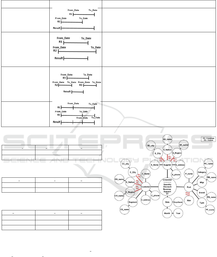
Table 5: Temporal operators.

Temporal operation Case Condition in query

Temporal union

WHERE MIN(R1.From_Date,R2.From_Date)<=

s.valid_date<MAX(R1.To_Date,R2.To_Date)

Temporal join

WITH CASE WHEN R1.From_Date >= R2.From_Date

THEN R1.From_Date ELSE R2.From_Date END as

min_date,

CASE WHEN R1.To_Date =< R2.To_Date THEN

R1.To_Date ELSE R2.To_Date END as max_date

WHERE min_date<=s.valid_date<max_date

Temporal difference

WITH CASE WHEN R1.From_Date >= R2.To_Date

THEN R1.From_Date ELSE R2.To_Date END as

min_date,

CASE WHEN R1.To_Date =< R3.From_Date THEN

R1.To_Date ELSE R3.From_Date END as max_date

WHERE min_date<=s.valid_date<max_date

Temporal aggregation

WHERE R1.From_Date<=s.valid_date<R1.To_Date

AND R2.From_Date<=s.valid_date<R2.To_Date

Table 6: Results of Query 1.

Customer ID City Name Sales Amount

Cust001 Paris 3700

Cust001 Lyon 3800

Table 7: Results of Query 2.

Product ID Category Name Sales Amount

Prod001 Fresh 1500

Prod001 Dairy 6000

Table 8: Results of Query 3.

City Name Category Name Sales Amount

Paris Fresh 1500

Paris Dairy 2200

Lyon Dairy 3800

2. For the dimension SUPPLIER, the assignments

of one hundred randomly selected suppliers

were changed on the hierarchical levels C CITY,

C NATION and C REGION. Thus, these suppliers

were assigned to two different levels according to

the two time intervals T

= [FD

= 01/01/1992,

T D

= 01/01/1996] and T

′

= [FD

= 01/01/1996,

T D

= 31/12/9999].

3. For the dimension PART, the SIZE attributes of

one hundred randomly selected products were

Figure 6: Logical schema for the SSB graph temporal DW.

changed. Thus, these products had two different

sizes; they had one size for the time interval T

= [FD

= 01/01/1992, TD

= 01/01/1995] and

another size for the time interval T

′

= [FD

01/01/1995, T D

= 31/12/9999].

We use the query Q3.3 from the SSB queries as an

illustrative example:

OPTIONAL MATCH (c:cc_city) <-[:c_c_name]-

(:c_city)<-[r1:customer_city]-(:customer)

<-[:order_customer]-(l:lineorder)-[:orde-

r_date]->(d:date),(s:sc_city)<-[:s_c_name]

Temporal Multidimensional Model for Evolving Graph-Based Data Warehouses

-(:s_city)<-[r2:supplier_city]-(s:supplier)

<-[:order_supplier]-(l)

WHERE r1.From_Date<=l.valid_date<r1.To_Date

AND r2.From_Date<=l.valid_date<r2.To_Date

AND 1992<= d.D_YEAR<=1997

AND (c.c_city="united ki1"

OR c.c_city="united ki5")

AND (s.s_city="united ki1"

OR s.s_city = "united ki5")

RETURN c.c_city, s.s_city, d.d_year,

SUM(l.lo_revenue) AS revenu

ORDER BY d.d_year ASC, revenu DESC

The previous query requires an aggregation of the

CITY levels of the dimensions CUSTOMER and SUP-

PLIER. Since these levels are temporally related to

the above dimensions, the query has been conditioned

according to the FD and TD parameters of these re-

lationships. Thus, we obtain a consistent result that

accurately reﬂects the state of the data. We were able

to apply the 13 queries proposed for the SSB in a tem-

poral format, and all of the results were veriﬁed. The

dataset, the commands for creating the GTDW and

all the queries that have been written in the CRL are

available at GTDW GITHUB.

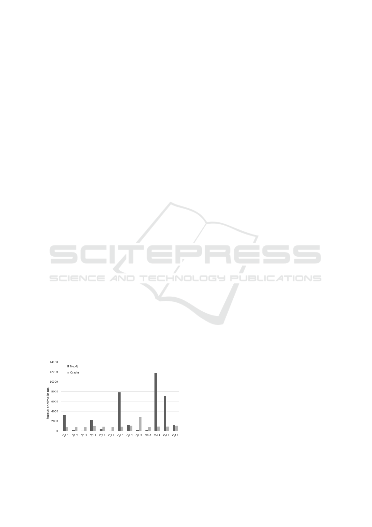
For the runtime performance study and due to

the lack of a baseline for scalable data warehouses,

we generated the same SSB schema using our graph

approach, spread over the entire validity period of

the data, and compared the execution times of the

13 queries on relational and graph approaches. The

dataset, the commands for creating the full graph DW

and all the queries are available at GSSB GITHUB.

The experimental procedure was performed on Win-

dows 10 Professional with an Intel(R) Core(TM) i7-

10700 CPU @ 2.90 GHz and 16.0 GB of RAM. Neo4j

4.4.5 was used for the graph approach and Oracle

11g was used for the relational approach. The exe-

cution times displayed in Figure 7 represent the aver-

age of ten executions for each query using the two

approaches (the same results were obtained on an

Ubuntu platform with the same conﬁguration).

Figure 7: Response times for SSB queries using the graph

and relational approaches.

We found through the results obtained that the

graph approach performed better for the queries Q1.2,

Q1.3, Q2.2, Q2.3, Q3.3 and Q3.4 (from 2x to 11x

better). The two approaches were quite close, with

the relational approach being slightly faster, for the

queries Q3.2 and Q4.3, and the relational approach

performed better for the queries Q1.1, Q2.1, Q3.1,

Q4.1 and Q4.2 (2x to 8x better). These differences

in the execution times of the response graph approach

depend on the ﬁlter factors (FFs), the number of di-

mensions and the number of edges to be covered. In-

deed, Neo4j can be very efﬁcient when the FF is low,

just as it can become less efﬁcient as the FF and the

number of dimensions increase, which implies that

many relations need to be browsed to carry out an

aggregation function; on the other hand, Oracle is

quite homogeneous in terms of the execution time of

the queries. However, in the context of temporal ap-

proaches, a performance study must be carried out on

the entire integration and storage process.

8 CONCLUSION

In this paper, we proposed a temporal multidimen-

sional model for multi-version data warehouses based

on a graph formalism. Temporal labelling has been

used for entities and the relationships between them

to allow the optimal management of data instances

and to preserve the evolutionary history of these data,

especially for changes in dimensions, in addition to

providing the capacity for schema evolution offered

by the concept of multi-versioning in DWs. We have

established rules for moving from a classical multidi-

mensional model to the temporal graph multidimen-

sional model, and an example of an instance and ex-

amples of temporal queries have been provided. We

have validated our approach with two use cases by

carrying out functional validation and runtime perfor-

mance experiments. We plan to carry out a perfor-

mance study of the entire integration process and fur-

ther study OLAP queries and graph cubes. In addi-

tion, we plan to carry out a study on advanced analy-

ses in graph models in order to utilise online analysis

to produce explanatory and predictive models.

REFERENCES

Ahmed, W., Zim

anyi, E., Vaisman, A. A., and Wrem-

bel, R. (2020). A temporal multidimensional model

and OLAP operators. Int. J. Data Warehous. Min.,

16(4):112–143.

Ahmed, W., Zim

anyi, E., and Wrembel, R. (2015). Tempo-

DATA 2023 - 12th International Conference on Data Science, Technology and Applications

ral data warehouses: Logical models and querying. In

Zim

anyi, E., Vansummeren, S., and Calders, T., ed-

itors, Actes des 11es journ

ees francophones sur les

Entrep

ots de Donn

ees et l’Analyse en Ligne, volume

B-11 of RNTI, pages 33–48.

Akoka, J., Comyn-Wattiau, I., du Mouza, C., and Prat, N.

(2021). Mapping multidimensional schemas to prop-

erty graph models. In Advances in Conceptual Mod-

eling – ER 2021, CMLS, St. John’s, NL, Canada, Oc-

tober 18–21, 2021, volume 13012 of Lecture Notes in

Computer Science, pages 3–14. Springer.

Benhissen, R., Bentayeb, F., and Boussaid, O. (2022).

GAMM: un mod

ele multidimensionnel agile

a base de

graphes pour des entrep

ots multi-versions. Revue des

Nouvelles Technologies de l’Information, Business In-

telligence & Big Data, RNTI-B-18:29–46.

Benhissen, R., Bentayeb, F., and Boussaid, O. (2023).

GAMM: graph-based agile multidimensional model.

In Gallinucci, E. and Golab, L., editors, Proceedings

of the 25th International Workshop on Design, Opti-

mization, Languages and Analytical Processing of Big

Data (DOLAP) co-located with (EDBT/ICDT), Ioan-

nina, Greece, March 28, 2023, CEUR Workshop Pro-

ceedings, pages 23–32. CEUR-WS.org.

Bliujute, R., Saltenis, S., Slivinskas, G., and Jensen, C. S.

(1998). Systematic change management in dimen-

sional data warehousing. In Proceedings of the Third

International Baltic Workshop on Data Bases and In-

formation Systems, Riga, Latvia. Citeseer.

Campos, A., Mozzino, J., and Vaisman, A. (2016). To-

wards temporal graph databases. arXiv preprint.

arXiv:1604.08568.

Debrouvier, A., Parodi, E., Perazzo, M., Soliani, V., and

Vaisman, A. A. (2021). A model and query language

for temporal graph databases. The VLDB Journal,

30:825–858.

Faisal, S. and Sarwar, M. (2014). Handling slowly chang-

ing dimensions in data warehouses. J. Syst. Softw.,

94:151–160.

Faisal, S., Sarwar, M., Shahzad, K., Sarwar, S., Jaf-

fry, S. W., and Yousaf, M. M. (2017). Temporal

and evolving data warehouse design. Sci. Program.,

2017:7392349:1–7392349:18.

Garani, G., Adam, G. K., and Ventzas, D. (2016). Temporal

data warehouse logical modelling. Int. J. Data Min.

Model. Manag., 8(2):144–159.

Golfarelli, M., Maio, D., and Rizzi, S. (1998). Concep-

tual design of data warehouses from E/R schema. In

Thirty-First Annual Hawaii International Conference

on System Sciences. IEEE Computer Society.

Golfarelli, M. and Rizzi, S. (2007). Managing late mea-

surements in data warehouses. Int. J. Data Warehous.

Min., 3(4):51–67.

Golfarelli, M. and Rizzi, S. (2011). Temporal data ware-

housing: Approaches and techniques. In Integrations

of Data Warehousing, Data Mining and Database

Technologies – Innovative Approaches. Information

Science Reference.

Golfarelli, M. and Rizzi, S. (2018). From star schemas to

big data: 20+ years of data warehouse research. In A

Comprehensive Guide Through the Italian Database

Research Over the Last 25 Years, volume 31 of Stud-

ies in Big Data, pages 93–107. Springer International

Publishing.

Inmon, W. H. (1992). Building the Data Warehouse. John

Wiley & Sons, Inc., USA.

Kimball, R. (1996). The Data Warehouse Toolkit: Practi-

cal Techniques for Building Dimensional Data Ware-

houses. John Wiley & Sons, Inc., USA.

Kimball, R. and Ross, M. (2013). The Data Warehouse

Toolkit: The Deﬁnitive Guide to Dimensional Model-

ing. Wiley, Indianapolis, IN, USA, third edition.

Kulkarni, K. G. and Michels, J. (2012). Temporal features

in SQL: 2011. SIGMOD Rec., 41(3):34–43.

Mendelzon, A. and Vaisman, A. (2000). Temporal queries

in OLAP. Proceedings of the 26th International Con-

ference on Very Large Data Bases, VLDB’00.

Phungtua-Eng, T. and Chittayasothorn, S. (2019). Slowly

changing dimension handling in data warehouses us-

ing temporal database features. In Intelligent Informa-

tion and Database Systems – 11th Asian Conference,

volume 11431 of Lecture Notes in Computer Science,

pages 675–687. Springer.

Poscic, P., Babic, I., and Jaksic, D. (2018). Temporal func-

tionalities in modern database management systems

and data warehouses. In 41st International Conven-

tion on Information and Communication Technology,

Electronics and Microelectronics. IEEE.

Saroha, K. and Gosain, A. (2015). Bi-temporal schema ver-

sioning in bi-temporal data warehouse. CSI Transac-

tions on ICT, 3:135–142.

Vaisman, A. and Zim

anyi, E. (2022). Temporal and Mul-

tiversion Data Warehouses, pages 373–436. Springer

Berlin Heidelberg, Berlin, Heidelberg.

Temporal Multidimensional Model for Evolving Graph-Based Data Warehouses