
Decomposition Heuristic for the Aircraft Sequencing Problem:
Impact on Mathematical and Constraint Programming
Joana Leite
1,2 a
, Rafael Guedes
3
and Diogo Queirós
3b
1
Polytechnic Institute of Coimbra, Coimbra Business School, Quinta Agrícola - Bencanta, 3045-231 Coimbra, Portugal
2
CMUC - Center for Mathematics, University of Coimbra, 3001-501 Coimbra, Portugal
3
Faculty of Engineering, University of Porto, 4200-465 Porto, Portugal
Keywords: Aircraft Sequencing Problem, Aircraft Landing Problem, Mixed Integer Programming, Constraint
Programming, Decomposition Heuristic, Parallel Processing.
Abstract: In this paper, we revisit the Aircraft Sequencing Problem (ASP), which consists of scheduling aircraft
landings respecting a pre-determined time window and separation criteria. ASP has several versions, with the
static single runway being the one with the longer solving times for the benchmark instances, for both mixed
integer programming (MIP) and constraint programming (CP) implementations. We considered this version
of the problem and addressed the possibility of using parallel processing to solve it. For this purpose, we
developed a heuristic for splitting the instances, which always guarantees a feasible solution that is the optimal
solution if a set of conditions is satisfied. The splitting allows for parallel processing, and opens the possibility
of using the best method to solve each subset of the partition obtained. To explore this feature, we also
analysed the performances of MIP and CP implementations and constructed a measure to point to the fastest
one. For the benchmark instances, the results show a time reduction over 50%, in the cases the optimal solution
is known, and an improvement of over 12% on the value of the best-known feasible solution, in the cases the
optimal solution is not known and running time has to be limited.
1 INTRODUCTION
The Airports Council International (ACI) World
Airport Traffic Forecasts 2022–2041 (ACI, 2023)
expects airports worldwide will see 153.8 million
aircraft movements by 2041.
As pointed out by Cohen and Coughlin (2003), a
common response to airport congestion by many
community leaders is to expand capacity by
constructing new runways and terminals. However,
airports expansions are costly, complex, and
controversial. At the same time, environmental and
geographic restrictions are also barriers to the
increase of airports logistics capacities. Hence, one
must use the existing capacities as efficiently as
possible in order to avoid flight delays and increase
the throughput.
So, prior the incursion on expansion planning and
construction, the problem of efficiently scheduling
the aircraft landings (and departures) should be
a
https://orcid.org/0000-0001-6828-9486
b
https://orcid.org/0000-0002-9972-496X
improved. Such problem is called Aircraft
Sequencing Problem (ASP) or Aircraft Landing
Problem, which is an important issue in air traffic
control.
In ASP, each plane to land has an optimal speed
(cruise speed) which is the most economic for that
plane. The target time of a plane is the time of landing
if it is flies at cruise speed. However, it may incur in
costs if air traffic control requires it to either slow
down, hold or speed up. This cost will grow as the
difference between the assigned landing time and the
target landing time grows, as illustrated in Beasley et
al. (2000).
The landing time must lie within a specified time
window, bounded by an earliest time and a latest time,
which depends on the plane. The earliest time
represents the earliest a plane can land if it flies at its
maximum airspeed. The latest time represents the
latest it can land if it flies at its most fuel-efficient
Leite, J., Guedes, R. and Queirøss, D.
Decomposition Heuristic for the Aircraft Sequencing Problem: Impact on Mathematical and Constraint Programming.
DOI: 10.5220/0012081500003541
In Proceedings of the 12th International Conference on Data Science, Technology and Applications (DATA 2023), pages 303-310
ISBN: 978-989-758-664-4; ISSN: 2184-285X
Copyright
c
2023 by SCITEPRESS – Science and Technology Publications, Lda. Under CC license (CC BY-NC-ND 4.0)
303

airspeed while holding (circling) for the maximum
allowed time.
Another aspect, that should be considered, regards
the separation time between planes. Separation times
depend on aerodynamic considerations. For example,
a Boeing 777X-9, with more than 70m of length and
wingspan, near 20m high and weighing 190ton
generates a lot more air turbulence and disruption
than a much smaller plane. So, a plane flying too close
behind could lose aerodynamic stability. For safety
reasons, landing a Boeing imposes larger delays so
that a second plane can land safely after it. In contrast,
a lighter and smaller plane generates little air
turbulence, thus a relatively short period goes by so
another plane can be landed.
As each aircraft has a preferred landing time, the
objective is to minimize the total delay costs for all
aircraft landings, while respecting the separation
requirements. The cost function approximates the
actual costs, namely fuel, maintenance, exhaust
emissions, and passengers missing their connecting
flights.
Over the last two decades several authors have
looked into ASP and its variations. Beasley et al.
(2000) studied the static case, an off-line case where
there is complete knowledge of the set of planes that
are going to land, setting the grounds for linear
programming and establishing what would become
the benchmark instances for this problem. Later on,
Fahle et al. (2003) combined both mixed-integer
zero-one programming (MIP) and constraint
programming (CP) to address the same problem. CP
revealed to have very powerful modelling
capabilities, but was by far the slowest method,
whereas MIP was the fastest exact optimization
method for instances with big time windows, but
showed difficulties in modelling non-linearities.
Different heuristics have been applied since to both
approaches. Veresnikov et al. (2019) and Zipeng and
Yanyang (2018) present excellent surveys, which
include a large number of heuristics, metaheuristics,
hybrid, and other algorithms to tackle the ASP. More
recently, Ahmadian and Salehipour (2020) proposed
a relax-and-solve algorithm, where the “relax”
procedure destructs a sequence of aircraft landings,
and the “solve” procedure re-constructs a complete
sequence and schedules the aircraft landings. The
algorithm was able to decrease the amount of time
needed to solve the benchmark instances.
In this work, we address ASP with two different
programming formulations, MIP and CP. We aimed
to compare the performances between these two
approaches and provide a set of indicators, or a single
metric, that could help decide which of the two
formulations is better for a given
instance. We should
also highlight here that we are dealing only with the
static case for a single runaway.
The rest of this paper is organized as follows: in
Section 2, we present the MIP and CP formulations
and the constraint formulation for the single runway
case; in Section 3, we explore a heuristic, based in a
naïve approach to fix planes, to boost MIP and CP
performance; in Section 4, we present the results,
compare and discuss the performances of both MIP
and CP formulations, with and without the aid of the
heuristic, and suggest a simple metric to help deciding
between the use of MIP or CP for ASP. Finally, in
Section 5, we draw some conclusions and purpose
future work.
2 PROBLEM FORMULATION
As already mentioned, to solve the ASP both MIP and
CP were used. In this section, we present the
respective formulations in detail, starting with the
introduction of the relevant notation.
Let 𝑛 be the number of planes to land. For each
plane 𝑖, with 𝑖∈
1,…,𝑛
, the following information
is known:
𝐸
earliest landing time for plane 𝑖,
𝐿
latest landing time for plane 𝑖,
𝑇
target/preferred landing time for plane 𝑖,
𝑆
minimum separation time required between
planes 𝑖 and 𝑗, if plane 𝑖 lands before plane 𝑗,
for 𝑗∈
1,…,𝑛
such that 𝑖𝑗,
𝑔
earliness cost, per unit of time, for landing
plane 𝑖 before its target time,
ℎ
tardiness cost, per unit of time, for landing
plane 𝑖 after its target time.
The values for times, namely 𝐸
, 𝐿
, 𝑇
and 𝑆
,
are non-negative integers. As for costs 𝑔
and ℎ
may
not be integers, but are non-negative and have, at
most, two decimal places. As mentioned in Beasley et
al. (2000), this has no significant loss of generality in
the ASL problem and, according to Fahle et al.
(2003), it is not a restriction in practice.
2.1 The MIP Model
Beasley et al. (2000) and Fahle et al. (2003) both
address the single runway static ASP using MIP, with
the same variables and basically the same
formulation.
The variables considered are, for 𝑖∈
1,…,𝑛
:
𝑥
landing time for plane 𝑖,
DATA 2023 - 12th International Conference on Data Science, Technology and Applications
304

𝛼
landing time deviation from the target time of
plane 𝑖, if it lands before target,
𝛽
landing time deviation from the target time of
plane 𝑖, if it lands after target,
𝛿
1 if plane 𝑖 lands before plane 𝑗
(𝑗∈
1,…,𝑛
;𝑖𝑗), and 0 otherwise.
However, the Beasley et al. (2000) formulation is
more detailed, separating planes in three sets, which
aids the solver to be used to obtain the optimal
solution faster with more complex instances.
Therefore, we adopt their formulation as the MIP
standard formulation:
Minimize
𝑔
𝛼
ℎ
𝛽
(1)
subject to, for all 𝑖,𝑗 ∈
1,…,𝑛
such that 𝑖𝑗:
𝐸
𝑥
𝐿
(2)
𝛿
𝛿
1 , for
𝑗
𝑖
(3)
𝛿
1 , ∀
𝑖,
𝑗
∈𝑊∪𝑉
(4)
𝑥
𝑥
𝑆
, ∀
𝑖,
𝑗
∈𝑉
(5)
𝑥
𝑥
𝑆
𝛿
𝐿
𝐸
𝛿
,∀
𝑖,
𝑗
∈𝑈
(6)
𝛼
𝑇
𝑥
(7)
0𝛼
𝑇
𝐸
(8)
𝛽
𝑥
𝑇
(9)
0𝛽
𝐿
𝑇
(10)
𝑥
𝑇
𝛼
𝛽
(11)
where
𝑈
𝑖,𝑗
∈
1,…,𝑛
| 𝐸
𝐸
𝐿
or
𝐸
𝐿
𝐿
or 𝐸
𝐸
𝐿
or
𝐸
𝐿
𝐿
and 𝑖𝑗
𝑉
𝑖,𝑗
∈
1,…,𝑛
| 𝐿
𝐸
and
𝐿
𝑆
𝐸
and 𝑖𝑗
𝑊
𝑖,𝑗
∈
1,…,𝑛
| 𝐿
𝐸
and 𝐿
𝑆
𝐸
and 𝑖𝑗.
2.2 The CP Model
Generally speaking, the CP formulation of a problem
can be closely related to the solver which is going to
be used, since the set of global constraints varies from
solver to solver. With that said, for the ASP, this does
not seem to be a very relevant issue, because the
separation time constraint that has to be enforced in
relation to all planes landing before a certain plane is
not easily implemented with global constraints.
Nevertheless, global constraints can be used as
redundant constraints to further increase efficiency.
The CP model adopted here for the single runway
static ASP, which we named CP standard
formulation, is based on the one proposed in Fahle et
al. (2003). The variables considered are, for
𝑖∈
1,…,𝑛
:
𝑥
landing time for plane 𝑖 → integer variable
with domain 𝐸
..𝐿
,
𝑐𝑜𝑠𝑡
costs induced by plane 𝑖 → integer
variable with domain 0..999999999,
𝑏
true if plane 𝑖 lands before target, and false
otherwise,
𝑝𝑝
true if plane 𝑖 lands before plane 𝑗
( 𝑗∈
1,…,𝑛
;𝑖𝑗 ) with plane 𝑗
respecting the separation time to plane 𝑖,
and false otherwise,
and the constraint set is:
minimize
1
100
𝑐𝑜𝑠𝑡
(12)
𝑏
true,i
f
𝑥
𝑇
false,i
f
𝑥
𝑇
, ∀𝑖∈
1,…,𝑛
(13)
𝑐𝑜𝑠𝑡
100𝑔
𝑇
𝑥
, i
f
𝑏
true
100ℎ
𝑥
𝑇
, i
f
𝑏
false
, ∀𝑖∈
1,…,𝑛
(14)
𝑝𝑝
true,i
f
𝑥
𝑥
𝑆
false,i
f
𝑥
𝑥
𝑆
(15)
𝑝𝑝
𝑝𝑝
, ∀𝑖,
𝑗
∈
1,…,𝑛
,𝑖
𝑗
(16)
allDif
f
𝑥
,…,𝑥
(17)
In the above formulation, some redundancy has
already been introduced. However, to further explore
the potential improvement in efficiency given by
redundant constraints and global constraints, we add
the following integer and interval variables, for
𝑖∈
1,…,𝑛
:
𝑠𝑡𝑎𝑟𝑡
lower bound of the interval for plane 𝑖 →
integer variable with domain
𝐸
𝑑
..𝐿
,
𝑒𝑛𝑑
upper bound of the interval for plane 𝑖 →
integer variable with domain 𝐸
..
𝐿
𝑑
,
𝑝𝑖𝑛𝑡𝑒𝑟𝑣𝑎𝑙𝑠
𝑠𝑡𝑎𝑟𝑡
,2𝑑,𝑒𝑛𝑑
minimal separa-
tion window for plane 𝑖 → interval variable,
where 𝑑min
,∈
,…,
𝑆
1, and the global
constraint:
NoOverlap
𝑝𝑖𝑛𝑡𝑒𝑟𝑣𝑎𝑙𝑠
(18)
Decomposition Heuristic for the Aircraft Sequencing Problem: Impact on Mathematical and Constraint Programming
305

3 THE PROPOSED APPROACH
For a set of 𝑛 planes, the difficulty in optimizing ASP
with MIP or with CP is, in some part, related to the
number of planes, since, the bigger the 𝑛, the more
variables and constraints are in the model. Thus, in
this section, we explore the possibility of dividing the
larger problem of landing 𝑛 planes into smaller
problems, in other words, into several ASP each with
a lower number of planes.
To do this, we start by introducing the notation
and convention used. We then present the two naïve
procedures which can lead to a feasible solution of the
ASP, without concern about optimization. Following
that, we briefly discuss a particular objective function
of the ASP. Finally, we present a heuristic approach
for the ASP where a feasible solution is found which
is very close or even equal to the optimal solution.
Staring with the notation, given a set of 𝑛 planes
to land, let
𝑇
,𝑇
,…,𝑇
be the 𝑛-tuple of target
times, where 𝑇
is the landing time of plane 𝑖, and
𝑥
,𝑥
,…,𝑥
be the 𝑛-tuple of landing times, where
𝑥
is the landing time of plane 𝑖. For simplicity and
without losing generality, in the following, we will
consider the coordinates of these 𝑛-tuples in
ascending order of the target time (i.e., 𝑇
𝑇
⋯𝑇
). Therefore, the coordinates in
𝑇
,𝑇
,…,𝑇
are not decreasing, but the same does not necessarily
happen with the coordinates in
𝑥
,𝑥
,…,𝑥
.
3.1 The Naïve Forward Procedure and
the Naïve Backward Procedure
The Naïve Forward Procedure (NFP) for the ASP is
based on the sequencing landing procedure known as
first-come-first-served (Bennell et al., 2011). It is a
very simple way to obtain a feasible solution for the
ASP, if the time window allows it. In NFP, the planes
are landed respecting the line-up determined by the
ascending ordination the target times (and, in case of
a tie, the first plane to land is the one with the highest
cost associated), and sequentially landing a plane on
the target time, if all separation times between that
plane and previous planes are respected, or as soon as
possible, otherwise. Let 𝐿
be the landing time of
plane 𝑖 obtained using NFP. Then, mathematically,
the landing times in NFP are given by:
𝐿
𝑇
(19)
𝐿
max
𝑇
,𝐿
𝑆
, for 𝑖2,…,𝑛.
(20)
The Naïve Backward Procedure (NBP) is
identical to NFP, but instead of landing the planes
starting with the one which has the smallest target
time, it begins by landing the one with the largest
target time, and proceeds backwards. Let 𝐿
be the
landing time of plane 𝑖 obtained using NBP. More
specifically, the landing times in NBP are given by:
𝐿
𝑇
(21
)
𝐿
min
𝑇
,𝐿
𝑆
, for 𝑖1,…,𝑛1. (22)
This procedure also provides a feasible solution
for the ASP, if the time window allows it.
3.2 Minimizing Deviations of the
Landing Times from the Target
Times
In the ASP, if we consider that the costs are all equal
(i.e., 𝑔
ℎ
⋯𝑔
ℎ
), minimizing the
objective function is equivalent to minimizing the
absolute deviations of the landing times from the
target times; more precisely, it is equivalent to
min
|
𝑇
𝑥
|
.
(23)
If a feasible solution can be obtained from the NFP
and/or the NBP, then
min
𝐿
𝑇
,𝑇
𝐿
(24)
is an upper bound of problem (23).
3.3 Decomposition Heuristic Procedure
For the particular case presented in the previous
subsection, it is possible to devise a way, using NFP
and NBP, to obtain the optimal solution in a shorter
time, if all separation times are less or equal to twice
the minimum separation times. To do this we apply
NFP and NBP, and we retain all planes such that
𝐿
𝐿
𝑇
(25)
for 𝑘∈
1,2,…,𝑛
.
It can be shown that, if we have a plane that
satisfies equation (25), then it is true that we can find
an optimal solution where:
i) this plane also lands on target;
ii) all the planes that have a smaller target time,
land before it;
iii) all the planes that have a larger target time,
land after it.
Therefore, the larger problem of landing the 𝑛
planes can be broken down into smaller problems,
separated by the planes that verify equation (25).
Depending on the separation times, but, for
DATA 2023 - 12th International Conference on Data Science, Technology and Applications
306

simplicity, let us focus in the case where the
separation times are close to each other, then these
smaller problems are independent from each other,
which allows to use parallel processing to run the
algorithms.
It is relevant to notice that this procedure can also
be applied to the more general ASP (in which costs
are not all equal), and, even though, in the general
case, optimality cannot be guaranteed, the solution
obtained for the ASP will be very close or even equal
to the optimal solution, especially if the values of all
landing costs are very close together and the
maximum separation time is less or equal to twice the
minimum separation time.
_______________________________
Decomposition Heuristic (DH) Procedure
1. Apply NFP to obtain 𝐿
,𝐿
,…,𝐿
(i.e., the
landing times when the plane with the lowest
target time lands on target and, if needed, the
others planes are pushed to forward times,
landing on or after target).
2. Apply NBP to obtain 𝐿
,𝐿
,…,𝐿
(i.e., the
landing times when the plane with the highest
target time lands on target and, if needed, the
others planes are pulled to previous times,
landing on or before target).
3. Determine the set of planes 𝑃 such that
𝐿
𝐿
𝑇
, for 𝑖∈
1,…,𝑛
.
4. If #𝑃0, then apply the MIP standard or the
CP standard procedure, and finish.
Otherwise, proceed to the next step.
5. Order the planes by ascending target times and
split this ordered set of 𝑛 planes into 𝑘
1
subsets using the planes in 𝑃.
The planes used to split are placed in all subsets
they determine, which can be one or two
subsets. If consecutive planes belong to 𝑃, then
they work as a whole.
6. In each subset:
– for all planes in 𝑃, update the earliest
landing time and the latest landing time to
the target time;
– for all planes not in 𝑃:
> if the subset starts with planes in 𝑃, say
𝑘 is the one with the highest target time
within 𝑃, then update the earliest landing
time of all planes not in 𝑃 to the
maximum between its provided earliest
landing time and the target time of plane
𝑘 plus the respective separation time
between these two planes;
> if the subset ends with planes in 𝑃, say 𝑘
is the one with the lowest target time
within 𝑃, then update the latest landing
time of all planes not in 𝑃 to the
minimum between its provided latest
landing time and the target time of plane
𝑘 minus the minimum of all separation
times.
7. To each updated subset and using parallel
processing, apply the MIP standard or the CP
standard procedure.
8. In an orderly manner, joint the 𝑘 solutions found
in the previous step.
9. Verify if all separation times are respected.
10. If the separation times are respected, then finish.
Otherwise, list the pair of planes that fail, and
finish.
_______________________________
In the DH procedure described, the step that most
contributes in running time reduction is the trimming
in the landing time windows executed in step 6, which
considerably decreases the window size for some
planes, and for the planes in 𝑃 reduces the window to
a single point.
4 RESULTS AND DISCUSSION
The algorithms presented in this paper were
programmed in Python and run on an Intel Core I7 –
8550U CPU @ 1.80 GHz (16 Gb RAM) for all
instances (1 to 13). To solve the mixed-integer and
constraint formulations of the problem to optimality
we used the PULP_CBC_CMD solver from the
PULP package (Roy et al., 2020) and the CP-SAT
solver from OR-Tools (Google LLC, 2020).
The 13 instances used here are the ones used by
Beasley et al. (2000), which are publicly available at
J.E. Beasley’s OR-Library (Beasely, n.d.). For the
discussion it is relevant to notice that we can divide
the instances in two groups that that have different
degrees of difficulty. Group 1 is composed of
instances 1 to 7, each characterized by a reasonable
low number of planes, with overlapped time windows
and almost all separation times symmetrical (i.e.,
𝑆
𝑆
). Group 2 is composed of instances 8 to 13,
that have a higher number of planes, ranging from 50
to 500, and almost no symmetrical separation times.
4.1 Assessing the Standard MIP and
CP Models
Table 1 summarizes all the results obtained from all
the models implemented in this study: MIP standard,
Decomposition Heuristic for the Aircraft Sequencing Problem: Impact on Mathematical and Constraint Programming
307
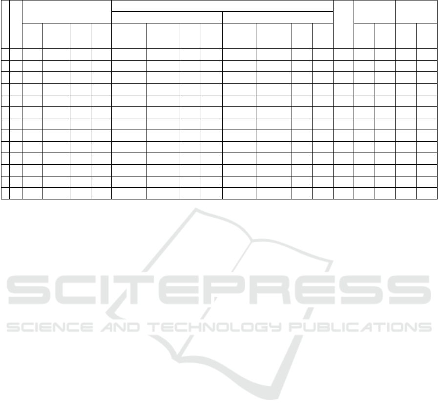
Table 1: Computational results.
Instance
No. Planes
MIP Standard
CP
No. Sets
from DH
MIP-DH CP-DH
Standard With Redundancy
Varia
-bles
Cons-
traints
BFS
Time
(s)
Conflicts Branches BFS
Time
(s)
Conflicts Branches BFS
Time
(s)
BKS
Time
(s)
BFS
Time
(s)
1 10 120 255 700* 0.56 189 781 700* 0.02 189 780 700* 0.05
1
700* 0.86 700* 0.04
2 15 255 450 1480* 2.47 5322 9434 1480* 0.37 5227 9272 1480* 0.29
2
1480* 3.29 1480* 0.36
3 20 440 750 820* 0.92 633 2742 820* 0.09 669 2839 820* 0.09
2
820* 0.49 820* 0.05
4 20 440 750 2520* 34.34 422779 519630 2520* 25.81 475257 585103 2520* 33.67
1
2520* 14.33 2520* 18.2
5 20 440 750 3100* 68.87 2476040 3090352 3100* 238.82 2549564 3176484 3100* 152.26
1
3100* 22.97 3100* 107.7
6 30 960 905 24442* 0.25 0 0 24442* 0.06 0 0 24442* 0.03
-
- - - -
7 44 2024 1587 1550* 4.72 41419 45691 1550* 6.03 80159 83531 1550* 6.24
-
- - - -
8 50 2600 4114 1950* 36.68 908848 1329678 1950 >3600 1574948 2408028 1950 >3600
4
1950* 1.11 1950* 0.22
9 100 10200 12219 6186 >3600 11113626 18639588 7521 >3600 4224066 7788409 8592 >3600
5
5633 >3600 5606 >3600
10 150 22800 25869 16779 >3600 7435701 13986412 16779 >3600 3210455 6255785 25137 >3600
5
13621 >3600 19349 >3600
11 200 40400 44584 14016 >3600 5292859 11728993 15574 >3600 3926510 8655811 16403 >3600
6
12592 >3600 21137 >3600
12 250 63000 68477 20144 >3600 3989610 9872690 31280 >3600 4232316 10430915 28397 >3600
11
16216 >3600 16296 >3600
13 500 251000 262552 47924 >3600 1719857 10074489 99575 >3600 2018402 11702868 90061 >3600
14
43853 >3600 53742 >3600
BFS – best-found solution; * optimal solution.
CP standard and with redundancy, MIP-DH and CP-
DH.
For each model, the best-found solution and
respective times are presented. Also, for MIP and CP
we chose to present the number of variables and
constraints created for each instance as an
approximation of the complexity level. We start by
briefly comment the global results and then present a
more detailed discussion in the following four
subsubsections.
From Table 1, it is clear that the DH method
applied with MIP or CP led to better solutions as well
as faster processing time. In addition, good (if not
optimal) feasible solutions are found early in the tree
search for a number of the instance, namely 9 to 13,
for which an optimal solution has not been found by
MIP or CP standard.
4.1.1 MIP and CP Standard
Upon comparing both models, MIP and CP standard,
it is possible to observe that CP has the best
performance, time wise, for the first four instances. It
is noteworthy the number of variables created by both
models in order to solve the problem.
When scaling the problem beyond the 44 planes,
MIP formulation outperforms CP. We should call the
attention towards instances 4 and 5. Although they
have a considerable low number of planes, another
particularly must be present that makes it harder for
CP to solve the problem (this is further discussed in
Section 4.2).
When entering in Group 2, no optimal solution is
found by both formulation below a time offset of
3600 seconds. Although the solutions found by MIP
and CP have close values, the best ones were always
accomplished by MIP.
It is relevant to notice that the values here
obtained and presented (i.e., the solutions) are equal
to those reported by Beasley et al. (2000) and Fahle
et al. (2003).
4.1.2 CP and CP with Redundancy
Redundancy is an important feature to be considered
when dealing with CP. When introduced, it has the
potential to reduce the difficulty of the problem at
hand by simplifying it. This is usually achieved
through domain reduction and, subsequently, search
space reduction.
With the use of a general constraint, in this case
NoOverlap from OR-TOOLS, we tried to improve the
CP performance through redundancy. Nonetheless, it
only seemed to have some effect on solving instance
5, where it was able to cut down by 36% the time
needed. Moving to Group 2, this strategy did not seem
to have much effect. In fact, the solutions obtained for
the objective function using this strategy were worse,
except for instances 12 and 13. For instances 9, 10
and 11, in the time given (i.e., 3600s), the standard
approach was able to produce better results than CP
with redundant constraints.
In light of these results, and not being a priority
objective of this work, we can only hypothesize on
the cause. Initially, the computational effort spent
reducing the problem is worthwhile, but becomes less
and less efficient. It will, eventually, stop
DATA 2023 - 12th International Conference on Data Science, Technology and Applications
308

compensating in terms of search space reduction and
not producing the best results.
Nevertheless, more attention should be given to
the redundancy topic. Firstly, a better and more
detailed design of the use of global restriction should
be done since these have the potential to help solving
the problem in shorter period of times. Also,
symmetry should be studied and understood how it
can be removed from the search step.
4.1.3 Evaluating the DH Procedure
The main objective of creating and introducing the
DH procedure was to decrease the amount of time
needed to solve the ASP (or reach a better value for
the objective function in the time given, 3600s) using
both MIP and CP formulation. As DH divides the
main problem in smaller groups, with strictly defined
time intervals and, consequently, less planes, one
should expect a decrease in the global difficulty.
In fact, analysing Table 1, we can verify that the
objective was accomplished.
From instance 1 to 3 there is no concrete
discussion to be done, as the problems were already
simple enough to be solved with the standard
formulations. Thus, DH did not bring any advantage
in the simple cases. Moving to instances 6 and 7,
given the fact that the combination of NFP and NBP
was not able to fix any plane, the DH could not be
applied. Instances 4, 5 and 8 saw their resolution time
being decreased considerably just to achieve the best-
found solution. Upon entering the set of instances
with more than 100 planes, the complexity increases
considerably. Since an output was to be given after
3600s, all the values obtained when DH was applied
were better than those obtained with MIP and CP
standard formulations. This means that if faced with
a situation where a solution is needed, with not
enough time to find the optimal, DH brings a
considerable advantage to the air traffic control.
Globally, for this set of instances, for the MIP
formulation, DH reduced in 70% the time needed to
find an optimal solution (instances 1 to 8) and 13%
the value of the objective function. Regarding the CP
formulation, DH reduced in 52% the time to find the
optimal solution and 32% the value of the objective
function.
4.2 The MIPvsCP Coefficient
The MIPvsCP coefficient was created to assess
whether an instance will be faster to solve and/or get
a lower value for the objective function, in a specific
model (MIP or CP), without the need of running the
instance on any of the two models.
The main goal here is, based on the properties of
an instance, decide to use either MIP or CP using
MIPvsCP coefficient, defined as followed:
MIPvsCP
1
𝑁
∑
𝜎
𝜇
∗𝑃
∑
𝑃
(26)
To design this coefficient, we took in
consideration three main aspects:
1. The number of groups within an instance (𝑁).
− To calculate the number of groups, we need
to sort, ascendingly, the planes in an instance
by their target times 𝑇
.
− Then, we calculate the difference between
the target times 𝑇
𝑇
of two
consecutive planes.
− If more than one plane has a difference lower
than the minimum separation time within the
instance and those planes are consecutive,
then, they stay in the same group.
2. The number of planes within each group 𝑖 (𝑃
),
which is raised to the power of two in order to
reinforce that the difficulty is exponentially
proportional to the number of planes within a
group, i.e., a group with six planes is more
difficult to solve than two times the difficulty of
a group with three planes.
3. The variation coefficient within each group 𝑖
, calculated by the quotient between the
standard deviation ( 𝜎
and the average
(𝜇
of the target time within the group 𝑖.
Furthermore, in order to get one value per instance
and be able to compare the metric between different
instances, we divide the sum of the variation
coefficients of each group by the sum of the number
of planes within the group powered by two. Finally,
we divide the previous value by the number of
groups. The lower the value obtained, higher the
complexity of the instance to be solved.
The results are shown in Table 2, where the
instance and the best model for that instance is stated,
then the number of groups formed for MIPvsCP
calculation, and then the MIPvsCP value.
Analysing Table 2, we can say that for these
instances, for a MIPvsCP coefficient above 0.18% we
recommend using the CP model, and below 0.15% we
recommend MIP.
For instances within 0.18% and 0.15%, we have
no evidence to support which one is better.
Lastly, both MIP and CP can achieve good
performance for instances without any group formed.
Decomposition Heuristic for the Aircraft Sequencing Problem: Impact on Mathematical and Constraint Programming
309

Table 2: MIPvsCP values for each instance.
Instance Best model Grou
p
s MIPvsCP
(
%
)
1 CP 1 0.71
2 CP 1 0.41
3 Both 0 -----
4 CP 2 0.18
5 MIP 3 0.11
6 CP 8 1.45
7 Both 0 -----
8 MIP 2 0.15
9 MIP 19 0.05
10 MIP 33 0.05
11 MIP 40 0.03
12 MIP 56 0.004
13 MIP 109 0.0016
5 CONCLUSIONS
ASP is a problem that air traffic control faces on daily
basis on different airports around the world, and, as
such, new ways to help solve the problems are
pertinent.
In this work, we addressed ASP using MIP and
CP, both well studied and formulated in the related
literature. The two main contributions were the
design of a decomposition heuristic procedure to
boost the performance of MIP and CP and the
development of a quick measure that points out to the
formulation to be used prior to running them.
From the results presented, five main outcomes
should be retained:
MIP is better for complex problems;
CP is faster for simpler problems;
DH procedure provides a heuristic able to get a
good solution (or even an optimal one) in a
faster way;
When MIPvsCP coefficient is above 0.18%,
CP formulation should be used, and when it is
below 0.15%, MIP is the better bet.
There are still some enhancements that can be
made, such as pre-processing in the way mentioned in
(Beasley et al. 2000) and, in the CP formulation,
exploring additional redundant constraints and the
usefulness of some symmetry-breaking constraints.
In the DH procedure, two improvements can be made:
add the MIPvsCP coefficient to guide the choice
between MIP and CP to solve the smaller problems,
and address the case where the DH procedure is not
able to produce a feasible solution because of the
separation times. Notwithstanding, an easy answer to
this last issue is the use of part of NFP and/or NBP
solutions.
ACKNOWLEDGEMENTS
We are grateful to Professor Daniel Castro Silva and
Professor Gonçalo Figueira for proposing this
problem and for constructive suggestions and
comments. Nonetheless, any errors remain our own.
The first author acknowledges that this work was
partially supported by the Centre for Mathematics of
the University of Coimbra - UIDB/00324/2020,
funded by the Portuguese Government through
FCT/MCTES.
REFERENCES
ACI. (2023). World Airport Traffic Forecasts 2022-2041.
https://store.aci.aero/product/aci-world-airport-traffic-
forecasts-2022-2041/
Ahmadian, M. M., & Salehipour, A. (2020). Heuristics for
flights arrival scheduling at airports. International
Transactions in Operational Research, 00, 1–30.
https://doi.org/10.1111/itor.12901
Beasely, J. E. (n.d.). J.E. Beasley’s OR-Library: Aircraft
landing. Retrieved December 14, 2020, from
http://people.brunel.ac.uk/~mastjjb/jeb/orlib/airlandinf
o.html
Beasley, J. E., Krishnamoorthy, M., Sharaiha, Y. M., &
Abramson, D. (2000). Scheduling aircraft landings - the
static case. Transportation Science, 34(2), 180–197.
https://doi.org/10.1287/trsc.34.2.180.12302
Bennell, J. A., Mesgarpour, M., & Potts, C. N. (2011).
Airport runway scheduling. 4or, 9(2), 115–138.
https://doi.org/10.1007/s10288-011-0172-x
Cohen, J. P., & Coughlin, C. C. (2003). Congestion at
Airports: The Economics of Airport Expansions.
Review, 85(3), 9–26. https://doi.org/10.20955/r.85.9-
26
Fahle, T., Feldmann, R., Götz, S., Grothklags, S., &
Monien, B. (2003). The aircraft sequencing problem.
Lecture Notes in Computer Science (Including
Subseries Lecture Notes in Artificial Intelligence and
Lecture Notes in Bioinformatics), 2598, 152–166.
https://doi.org/10.1007/3-540-36477-3_11
Google LLC. (2020). ortools (Version 8.1.8487) [Python
library]. https://pypi.org/project/ortools
Roy, J. S., Mitchell, S. A., & Peschiera, F. (2020). PuLP
(Version 2.4) [Python library]. https://pypi.
org/project/PuLP
Veresnikov, G. S., Egorov, N. A., Kulida, E. L., & Lebedev,
V. G. (2019). Methods for Solving of the Aircraft
Landing Problem. I. Exact Solution Methods.
Automation and Remote Control, 80(7), 1317–1334.
https://doi.org/10.1134/S0005117919070099
Zipeng, L., & Yanyang, W. (2018). A Review for Aircraft
Landing Problem. MATEC Web of Conferences, 179, 1–
6. https://doi.org/10.1051/matecconf/201817903016.
DATA 2023 - 12th International Conference on Data Science, Technology and Applications
310
