A Flood Prediction Benchmark Focused on Unknown Extreme

Events

Dimitri Bratzel, Stefan Wittek and Andreas Rausch

Institute for Software and Systems Engineering, Clausthal University of Technology,

Arnold-Sommerfeld-Str. 1, Clausthal-Zellerfeld, Germany

Keywords: Machine Learning, Flood Prediction, Benchmark, Dataset, Unknown Events.

Abstract: Global warming is causing an increase in extreme weather events, making flood events more likely. In order

to prevent casualties and damages in urban areas, flood prediction has become an essential task. While

machine learning methods have shown promising results in this task, they face challenges when predicting

events that fall outside the range of their training data. Since climate change is also impacting the intensity of

rare events (i.e. by heavy rainfall) this challenge gets more and more pressing. Thus, this paper presents a

benchmark for the evaluation of machine learning-based flood prediction for such rare, extreme events that

exceed known maxima. The benchmark includes a real-world dataset, the implementation of a reference

model, and an evaluation framework that is especially suited analysing potential danger during an extreme

event and measuring overall performance. The dataset, the code of the evaluation framework, and the

reference models are publicated alongside this paper.

1 INTRODUCTION

Global warming not only leads to a rise in

temperature but also causes an increase in the

frequency and intensity of extreme weather events.

Floods are one such example of an event affected by

this trend (Alfieri et al., 2017).

In order to mitigate the negative impact of floods,

accurate and timely predictions of flood events are

critical. Predictions made 2-3 hours in advance can

provide crucial warning time to allow evacuation and

the implementation of preventative measures, thereby

reducing the damage caused by floods.

Artificial neural networks (ANN) and other

machine learning (ML) methods have shown

promising results in the prediction of flood events

(Goymann et al., 2019). However, a major challenge

in flood prediction is the issue of unknown extreme

events. If the precipation or the resulting water levels

exceed previous records, the ML algorithm is forced

to extrapolate – i.e., to do predictions outside of the

range of its training data. Many ML algorithms,

especially ANN, are known to perform poorly in

extrapolation scenarios (Minns and Hall, 1996).

Another factor that complicates unknown extreme

events is the rare occurrence of even the known

extreme events in the training set. This makes

predictions even more challenging.

These challenges are becoming increasingly

relevant with the effects of climate change, which are

likely to lead to an increase in the frequency of

record-breaking heavy rain and, consequently floods

in the future.

Despite the importance of this issue, existing

works on the extrapolation of ML-based flood

predictions are limited, with most studies focusing on

performance within the range of the training data.

While public datasets on water levels exist, they are

missing a framework for actual comprehensive

evaluation as well as a focus on unknown events and

extrapolation.

In this paper, we provide a benchmark based on

the city of Goslar in Germany, focusing on the

aforementioned challenges in flood predictions. This

benchmark case is particularly important since it is

located near the Harz region, a mountainous area in

Lower Saxony. Areas like this are suspected of

suffering from this increase in flood events as a result

of global warming (Allamano et al., 2009).

This benchmark includes the real-world dataset

spanning about 14 years and including one big flood

event as well as an evaluation framework focused on

the performance of these unknown situations. We

Bratzel, D., Wittek, S. and Rausch, A.

A Flood Prediction Benchmark Focused on Unknown Extreme Events.

DOI: 10.5220/0012081700003546

In Proceedings of the 13th International Conference on Simulation and Modeling Methodologies, Technologies and Applications (SIMULTECH 2023), pages 267-278

ISBN: 978-989-758-668-2; ISSN: 2184-2841

 2023 by SCITEPRESS – Science and Technology Publications, Lda. Under CC license (CC BY-NC-ND 4.0)

267

also provide a reference implementation using a

Long-Short-Term-Memory (LSTM) model. For the

evaluation framework as well as for the reference

implementation, code is provided

This allows other researchers to test their ML-

based flood prediction approaches with respect to

unknown events and compare the performance with

our baseline implementation.

The paper is structured as follows. After stating

the related work in section 2, section 3 gives a

detailed description of the data set. Section 4

describes the predictiv task definded based on this

dataset. Section 5 contains the evaluation framework,

incuding an event focused framework (section 5.1)

and a variety of metrics applied to the overall

prediction quality (section 5.2). In section 6 a

reference precitive model is described which is

evaluated using the framework in section 7.

2 RELATED WORKS

The discussed related work in this section can be

separated as follows: The forecast of a flood event

through ML, dealing with unseen events, datasets,

and mainly used framework for evaluating

hydrological models.

The ML-Based Flood Prediction

An extensive range of research has been done on

forecasting a high-water event. Usually, these papers

differ in hydrogeological features or the ML-

technology that was used to forecast the flood event.

This leads to the differences in the range of the

forecasting window, the data quality and quantity,

and the event that needs to be forecasted. Since ANN

offers advantages such as rapid development, low

execution time, the parsimony of data requirements

and a substantial open-source community

(Shamseldin, 2010), many works are using this

technique. Riad et al. discuss the forecast of a flood

event with a one-layer artificial neural network on

data collected in the Ourika basin in Morocco from

1990-1996 (Riad et al., 2004). Shameseldin et al.

apply the Multi-Layer Perceptron (MLP) model for

the Nile River in Sudan. The model considers data

such as rainfall index and seasonal expectation

rainfall index, and other meteorological input

information (Shamseldin, 2010). A similar

application of MLP was used in the region of Greater

Manchester, where the application of MLP was

justified because this technique is more suitable for

https://gitlab.com/tuc-isse/public/flood-benchmark

finding patterns and trends in complex data than

regular statistical models and algorithms (Danso-

Amoako et al., 2012). Although Danso-Amoako et

al., in their work, do not forecast the future status of

water level or similar, they predict the actual risk of

dam failure by creating a data-driven surrogate model

with using a MLP model. Very different is the case in

catchments with open water, for example, coastal

areas, where different sources may cause the

occurrence of extreme storm surges. In their work

Kim et al. discuss these effects of the surge and test

them on a MLP model to predict the surge in the

coastal region of Japan in Tottori (Kim et al., 2016).

Although the results are promising, the target of the

forecast is so-called "after-runner surge”, which

occurs 15-18 hours after a typhoon. Therefore, two

important pieces of information are used for the

forecast: the quantitative description of the typhoon

and the knowledge that an extreme surge event is very

likely to occur within the next 18 hours. A

comparison of the performance of different

techniques: MLP, Adaptive Neuro-Fuzzy Inference

System (ANFIS) and empirical models, on a huge

area of Peninsular Spain is presented in (Jimeno-Sáez

et al., 2017). A good systematic overview of the ML-

based prediction was done in (Mosavi et al., 2018)

where most common ML techniques are explained

and their application in different areas datasets and

forecast horizons are presented.

Prediction of Extreme Events

Despite the good results in forecasting weather

phenomena, most of the works deal with problems in

finding a pattern and recognizing an event that has

already happened in the past. The anomalous

behaviour of Artificial Neural Networks on

forecasting unseen events was observed in (Minns

and Hall, 1996), where the ANN performed very well

on test data that had the same minimal and maximal

values but could not overcome the maximal values in

the test set where the flood event had higher values

than the ones that could be observed on training data.

The authors concluded that MLP tends to recall seen

values but has problems generalizing if the flood

event shows higher values than the training data. To

solve the problem in (Hettiarachchi et al., 2005), the

solution of the so-called Estimated Maximum Flood

(EMF) was presented. In this case, the authors used

additional domain knowledge to generate artificial

data where an extreme event appears. This extreme

event is much higher than ever observed empirical

data with a probability higher than zero. The problem

was also observed and discussed in (Xu et al., 2020)

SIMULTECH 2023 - 13th International Conference on Simulation and Modeling Methodologies, Technologies and Applications

268

where the general problem of extrapolation of ANN

was analysed and theoretical and empirical evidences

were given that simple ANN does not predict

properly when values are out of the range of the

training sample. Whereas (Pektas and Cigizoglu,

2017) observe the ANN behaviour in the hydrology

during minima and maxima of the dataset that are out

of the training sample. (Goymann et al., 2019)

presented in their work in the catchment Goslar the

forecast of the flood event from 2017. Facing a

similar problem with LSTM-ANN, the authors

provided a classification-based approach. Therefore,

the result was a value of one if it was expectable that

a flood event in the next two hours could appear or

zero if no flood event was expected.

Flood Prediction Metrics

To evaluate the prediction models, several metrics

were used. This includes well-known, mean-based

metrics like root mean squared error (RMSE)

(Dtissibe et al., 2020; Jimeno-Sáez et al., 2017;

Mulualem and Liou, 2020), normalized root mean

square error (NRMSE) (Kim et al., 2016), mean

absolute and relative error (MARE) (Dtissibe et al.,

2020; Riad et al., 2004) also indices like the

correlation coefficient (CC) (Kim et al., 2016) and

coefficient of determination (R²) (Danso-Amoako et

al., 2012; Jimeno-Sáez et al., 2017; Riad et al., 2004;

Shamseldin, 2010). The main disadvantage of mean-

based metrics is that even significant forecast errors

decrease with the increasing number of right-

predicted values. This is a problem in big datasets

where an extreme, rare event should be predicted. The

paper (Krause et al., 2005) discusses several

efficiency criteria for the hydrological model. The

leading critique is that the Nash-Sutcliffe efficiency

(NSE) and the index of agreement (IoA) are sensitive

to errors in the peaks and less sensitive to systematic

errors in lower regions. By modifying the metrics,

authors propose how these metrics could be used as a

benchmark to evaluate errors in lower and higher

regions.

During the research, no related work could be

found that could fulfil the requirements for the

application in the catchment area of Goslar for the

forecast of values during high water levels, such as:

show difference of prediction versus Ground Truth,

robustness against growing number of predicted

values, explanation of errors (systematic error or

outlier), exact focus on the performance during

critical time (flood event).

Therefore, we present a benchmark that includes

the dataset of a rare extreme flood event, an

evaluation framework with event-focused evaluation

Figure 1: Geological overview of catchment Goslar (City

Goslar, Goymann, et al. 2019).

framework and modified overall metrics and the

example of the application of residual LSTM-Neural

Network on the problem of flood forecast in 2, 3 and

4 hours.

3 GOSLAR REGION DATASET

The catchment area of interest is the city of Goslar

and the high ground part from the settlement in south-

west (Figure 1). The river “Gose” (highlighted in

purple) that was responsible for the flood event in

2017 could be measured at station Sennhuette (D)

since the artificial under-earth connection between

the dam “Granetalsperre” at (B) and the river Gose at

Sennhuette (D) needs to be considered. As additional

input for the sudden rainfall, the weather stations (A)

Hahnenklee and (B) Margaretenklippe are available.

The river stream goes from the Southwest to the

city in the Northeast; therefore, the sensors are

essential to catch early data for sensing actual level of

the Gose, that enter the city centre at (D), the latest

point for measuring the water level before the city.

Granetalsperre (C) and Sennhuette (D) measure

the actual level of the water in [cm]. The current of

the water stream in [m³/s], which is also part of the

collected data, is not measured directly but is

automatically derived from this level and mixed

formal and parametrical model from

Harzwasserwerke GmbH during data collection. The

weather stations collect the rainfall in [l/m²]. The data

collection of all sensors happens every 15 minutes.

A Flood Prediction Benchmark Focused on Unknown Extreme Events

269

Table 1: Statistical overview of collected data.

Figure 2: Split in training and test data.

The data set consists of 514176 samples in the

time range from 01.11.2003 until 30.06.2018. In the

statistical description (Table 1), it can be observed

that the Sennhuette reaches its maximum value at

170.4 [cm], whereas the upper quartile is 9.8[cm].

This can be explained by the dataset that includes the

flood event from 2017 in Goslar (Figure 3).

Figure 3: Data during flood event 2017, Goslar.

Thus, a similar effect can also be observed in the

other data but the rainfall, where 75% of the data is 0.

The situation where quartiles are very close to each

other but relatively far away from the maximum value

and the maximum value cannot be considered as an

outlier; we call extreme, rare event. In the case of

Sennhuette the maximal value is almost 17 times

bigger than the upper quartile and cannot be reduced

as an outlier since this is the actual value that needs

to be predicted properly.

4 PREDICTIVE TASK

The hydrogeological experts of the catchment of

Goslar agree that with the view on the growing

importance of global climatic changes, the prediction

of high-level water events will grow, since the risk of

unexpected and intense rainfalls will grow. To allow

emergency services to activate the protection

procedure and warn the population of the catchment,

a prediction of at least 120 minutes is required.

Moreover, emergency services ask for immense

forecast horizons like 180 minutes (3 hours) and 240

minutes (4 hours).

Even though previous work of the Institute of

System Engineering at the Technical University of

Clausthal shows a promising and robust forecast for

the warning of extreme events that could meet the

requirements (Goymann et al., 2019), show that

despite accurate predictions of the water level, ANNs

work poorly during an extreme event. Although the

poor performance of regular ANN on unseen, rare

events is known, no dataset could be found that

Granetalsperre

[l/m²]

Hahnenklee

[l/m²]

Margarethenklippe

[cm]

Margarethenklippe

[m³/s]

Sennhuette

[cm]

Sennhuette

[m²/s]

coun

514176 514176 514176 514176 514176 514176

mean 0.03 0.04 10.40 0.12 7.98 0.11

std 0.19 0.21 5.84 0.20 6.26 0.20

min 0.00 0.00 3.70 0.01 1.50 0.01

25% 0.00 0.00 6.60 0.04 4.00 0.03

50% 0.00 0.00 8.70 0.07 6.00 0.05

75% 0.00 0.00 12.10 0.13 9.80 0.12

max 25.40 24.50 160.60 12.50 170.40 16.68

SIMULTECH 2023 - 13th International Conference on Simulation and Modeling Methodologies, Technologies and Applications

270

represents the problem correctly. Therefore, the

discussion about the evaluation of the performance of

models to forecast extreme, rare, and unseen events

could not make progress, which is demanded by

global climatic changes and concepts of safety

concerns.

For the training, 70% of the data can be used and

30% for testing. Even though more data could be used

for predicting the extreme event, it must be

considered that the extreme event must be a part of

the test set (Figure 2) and operations like shuffling are

only allowed to do after the split operation.

Therefore, the contribution of this work is a

benchmark for predictive models containing the data

set from the catchment area of Goslar including one

extreme event, an event-focused evaluation

framework and a set of adapted overall metrics.

The data, source code of the evaluation

framework and reference implementations of models

for 2-, 3- and 4-hours forecast are available as a git

repository:

https://gitlab.com/tuc-isse/public/flood-benchmark.

5 EVALUATION FRAMEWORK

The presented evaluation framework consists of an

event-focused evaluation framework and a set of

overall metrics suitable for evaluating the models.

The event-focused part gives an insight on the

performance of the model if applied to events that

exceed this training horizon. In contrast the overall

metrics allow the assessment of the model in general,

without this focus.

5.1 Event-Focused Framework

As discussed in previous chapters, a sudden high-

water event causes serious danger to the environment

of the catchment. Also, we discussed how average-

based metrics underestimate errors in regions with

lower values. Therefore, a framework for evaluating

predictive models was created that defines potential

danger events and allows the framework to be

adjusted to local hydrogeological conditions and

safety concerns.

The schematic visualization of the event-focused

framework is presented in Figure 4. The analytical

evaluation of a situation is as follows: dangerous

floods seem very likely when the water level rises, as

a drop in the measurements might indicate a

mitigation of the situation. Clusters where a constant

rise of the level 𝑦 is observed represent a severe

potential danger.

Let 𝑇



𝑡∈ℕ



be a set that represents the number

of time points where the measurements of the dataset

were made. The time points where the level is rising

can be described as:

𝑇







𝑡∈𝑇

𝑦



𝑦





(1)

Furthermore, the rising level is usually only

dangerous after overcoming a certain level of interest

𝛽 , which is specific to each catchment. The

measurements over this lowest level of interest can be

defined as

𝑇



𝑡∈𝑇



𝑦



𝛽

(2)

The time point where relevant measurements were

taken can be separated into three sets

𝑇



𝑇



∪𝑇



∪ 𝑇



(3)

Since the exact value is not needed in the

application scenario, a certain level of tolerance 𝑏 is

introduced.

𝑇



𝑡∈𝑇



𝑦



𝑦



𝑏

(4)

Describes the time points where forecasted values

are acceptable and can be considered as correct.

𝑇



𝑡∈𝑇



𝑦



𝑦



𝑏

(5)

Are time points of overestimation of the model

which could cause a potential false alarm.

𝑇



𝑡∈𝑇



𝑦



𝑦



𝑏

(6)

Are time points of underestimation of the model

where a potential flood alert could have been

overseen. These points are more critical than

overestimation since the consequences of a false alert

are less critical than the consequences of an overseen

flood event. The event-focused evaluation framework

was done by the definition of 𝜷𝟒𝟎 𝐜𝐦 as level

where the dangerous flood can appear, and the

acceptable variance of the prediction is 𝒃𝟏𝟎 𝐜𝐦.

Both values have been consolidated with the safety

concept of the city of Goslar.

These values can be interpreted accumulated as

the number of time points where the model forecasted

correct values or under- or overestimated the values

during a flood event. Also, the interpretation of

potential annual or relative right and false predictions

can be made. This is especially useful when

comparing models on datasets with different sizes.

The relative metrics are based on the amount of

all events:

A Flood Prediction Benchmark Focused on Unknown Extreme Events

271

Figure 4: Schematic visualisation of the event-focused framework.

𝑇



|𝑇



|𝑇





𝑇





𝑇

 

(7)

𝑇







|𝑇



𝑇



(8)

𝑇







|𝑇



𝑇



(9)

𝑇







|𝑇



𝑇



(10)

The annual comparison metrics have as a basis the

number of years in which the relevant events were

observed.

𝑦𝑒𝑎𝑟s 𝑜𝑏𝑠𝑒𝑟𝑣𝑒𝑑

𝑎𝑚𝑚𝑜𝑢𝑛𝑡 𝑜𝑏𝑠𝑒𝑟𝑣𝑒𝑑 𝑒𝑣𝑒𝑛𝑡𝑠

24  4  365

(11)

𝑇







|𝑇



𝑦𝑒𝑎𝑟𝑠

𝑜𝑏𝑠𝑒𝑟𝑣𝑒𝑑

(12)

𝑇







|𝑇



𝑦𝑒𝑎𝑟𝑠_𝑜𝑏𝑠𝑒𝑟𝑣𝑒𝑑

(13)

𝑇







|𝑇



𝑦𝑒𝑎𝑟𝑠_𝑜𝑏𝑠𝑒𝑟𝑣𝑒𝑑

(14)

While this measure gives a good comparative

overview of the performance of different models in

the predictive task, an interoperable metric related to

the actual probability of missing dangerous events is

still missing. For the example, a value of

𝑇

_

12 can be understand a mean of 12

potential flood events per year, that would not be

predicted correctly by the model. But there is no

information on how cluttered this missed floods are.

It is possible that these 12 events are spread out

evenly across this year, meaning that only a single

prediction for only a single 15 min interval is wrong

every month. This would be a neglectable error,

because all other prediction around this error would

be correct and correctly implying an incoming flood,

thus only reducing the warning time by 15 minutes.

In the other extreme these 12 events could indeed be

aligned in a single chain of errors hiding the flood for

3 hours. Also, the mean over the duration of observed

years may have a high variance, with some years

aggregating huge singe blind spots.

To tackle this issue, we added the statistic of

chains of underestimated levels (events in 𝑇



) as

an additional metric. A chain in this context is defined

as a subsequence of model predictions out of the

ordered set of all model predictions in which all

elements are within 𝑇



. Intuitively speaking,

how often the model underestimated a potential flood

event in a row. If a chain is broken by a correct

prediction, the parts are counted as different chains.

As a metric, we record the length of all chains

longer than a single element, and the length of the

longest chain, indicating the longest “blind spot” that

the model would have in the context of a warning

system.

5.2 Overall Metrics

To observe the performance of the model in all

regions, outside and during the extreme event, the

following overall metrics were adapted and applied

(Krause et al., 2005):

r: Bravais Pearson Correlation Coefficient (BP),

where one means that there is a perfect correlation

SIMULTECH 2023 - 13th International Conference on Simulation and Modeling Methodologies, Technologies and Applications

272

between the observed values O and the predicted P,

and zero when no correlation could be found. The

correlation coefficient could be used as an additional

indicator, but this coefficient is unsuitable for making

judgments about the size of the error.

r

∑

O



OP



P







∑

O



O









∑

P



P







(15)

E : Nash–Sutcliffe Efficiency (NSE) has,

according to Krause et al., low sensitivity to

systematic errors in lower regions and high

systematic errors in peaks of prediction.

E1

∑



P











∑

O



O







(16)

E

∞

E  0

total fit

no fit

worse than average

(17)

With the range E ∈1:  ∞ it can be interpreted as

follows:

d: Index of Agreement (IoA) faces the same

tendency to overrate errors in peaks and underrate

errors in lower regions.

d1

∑



P











∑

P



OP



O







(18)

With the range d∈1: 0 , the interpretation of the

model is as follows: d

1: total fit

0: no fit



: Modified Nash–Sutcliffe Efficiency and



modified Index of Agreement were alternated

to be more sensitive in lower regions when the

modification value J is smaller than two. In order to

focus on peaks, the factor J should be alternated to

values higher than 2. In this work, mainly the value

J3 was used.



 1 

∑|



 P









∑

O



 O







(19)



1

∑|



P









∑

P



OP



O







(20)

Because the event-focused framework is mainly

focused on rare, extreme events and the discussed

overall metrics are adjusted to observe prediction

errors in peaks, the systematic errors in lower regions

could rise and give the observer overall wrong

predictions. This could damage the reputation of the

prediction model so that emergency services would

only trust the values in higher regions where the

model would give better results. To compare the

overall prediction in lower regions, the modified

Nash–Sutcliffe Efficiency and modified Index of

Agreement with J2 should be used or as

suggested, relative derivation of both these metrics.

The overall framework shows in all metrics a

perfect fit. Meanwhile, all metrics show a poor result

in absolute negative correlation (Figure 5).

Figure 5: Negative linear correlation.

Figure 6: Evaluation with the high and low differences in

peak.



1

∑





P











∑





O









(21)



1

∑





P













∑



P



OP



O









(22)

In this framework, the relative metrics were

chosen to observe lower regions since they have

shown less sensitivity to small error changes.

Figure 7: Total linear correlation.

A Flood Prediction Benchmark Focused on Unknown Extreme Events

273

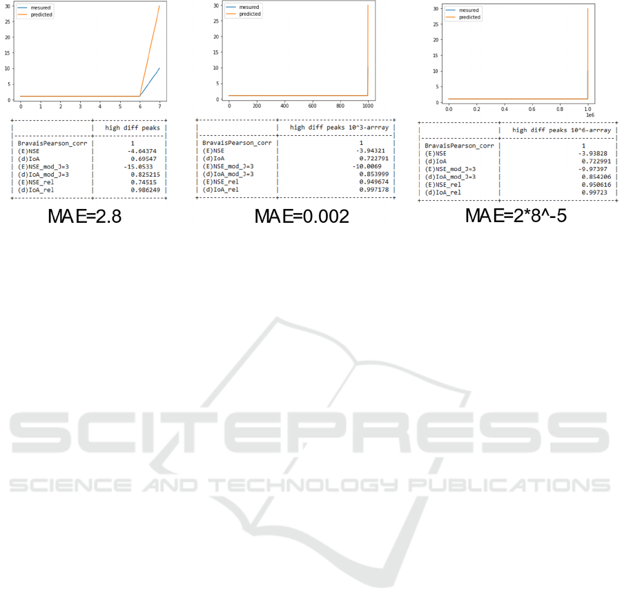
Figure 8: Rising number of compared values.

To observe the behaviour of the overall metrics,

different situations were modelled. In the first

example, the observed values equal the measured

OP (Figure 7).

Two situations are modelled to observe the effect

of error during peak, where all measured and

predicted values are equal but one (Figure 6). In the

first situation, the last value’s absolute error is 5; in

the second situation, the error of the peak is 20. The

metrics clearly show that NSA and IoA are sensitive

to the peak in the first situation and show the error

change in the peak in the second situation. The

modified NSA and IoA show similar results, and the

relative NSA and IoA show that model performs well

in lower regions. In all modified, relative and original

metrics, IoA shows more stability, whereas NSA

seems to be more sensitive.

The overall metrics generally show minimal

sensitivity to the growing number of predicted values

compared to the error. Unlike average-based metrics,

the error did not approach zero, even with very high

data. To observe the stability of the metric due to the

growing number of measurements, the situation with

an absolute error of 20 in the peak was alternated by

growing from 8 to 10^3 and 10^6 measurements

(Figure 8). The original and modified metrics could

sense the error in the peak even when the model is

improving due to the growing number of correct

predicted values in the lower region. For the lower

region, the relative metrics show a good performance

of the estimated values and are improving with the

growing number of equal measurements. Also

remarkable is the stability of all alternations of IoA in

these situations. In all these situations the BP

coefficient is failing to show any changes due to a

perfect correlation. Meanwhile, the Mean Absolute

Error (MAE) shows clearly how a relatively

significant error in a small dataset could lose

importance with the growing size of the data.

6 REFERENCE MODELS

The criteria for a successful prevention of more

significant damages from the sudden flood event in

Goslar requires a prediction of the flood at least two

hours in advance. Furthermore, rescue task forces

could improve their actions with the larger forecast

horizon. The results show that the forecast of 4 hours

in the observed catchment is possible. Therefore,

three models were generated with 2, 3 and 4 hours of

the forecast horizon. For all 3-time horizons two

architectures were tested; a simple LSTM-ANN with

32 neurons in each of four layers and a residual

LSTM-ANN with 8 residual blocks and 6 neurons in

each layer. All models take as input a series of 32 last

observed values from each sensor, presented in

Section 3, except from the data from Sennhuette and

gives back a forecast of the value of data stream

Sennhuette in 8, 12 or 16 future data points (2, 3 or 4

hours).Additional features were extracted to improve

the model performance. The 2- hours model includes

the gradient of the input of Sennhuette of one timestep

(in the past). In 3- and 4-hour models, a gradient of

192 timesteps (in the past) for Sennhuette and the area

under the curve for each of the two rainfalls were also

calculated for the past 96 timesteps.

In the tests, the residual LSTM neural network

outperformed the regular LSTM and the MLP of

different architecture in forecasting the values during

the extreme, unseen event. This might be explained

by the capability of the residual ANN architectures to

bypass input to the over layers. Meanwhile, in the

regular ANN, the information is passed from the

SIMULTECH 2023 - 13th International Conference on Simulation and Modeling Methodologies, Technologies and Applications

274

previous layer to the following. The residual neural

network gives to one hidden layer the information

that was generated by its direct predecessor and the

information from one of the predecessors or even

from the input layer. This reduces the risk of

overfitting, where neuronal connections that seem to

be unimportant are assigned lower weights and

important new information is ignored.

The validation split of the training data was done

with a pre-defined function of Keras-TensorFlow API

with 20%. The training was done for a maximum of

30 epochs with the possibility of early stopping and a

batch size of 265. The data was scaled using the

method StandardScaler, from the library sklearn.

7 RESULTS

As mentioned before, the evaluation framework

should be applied in two stages: the analysis of the

defined rare–extreme event via the event-focused

evaluation framework and the model's overall

performance in lower and upper regions of the

prediction via the overall metrics framework.

Therefore, in the next two chapters, an evaluation of

the residual LSTM-ANN is discussed and the

comparison with the performance of the simple

LSTM-ANN is done.

Table 2: Event focused evaluation of the LSTM-residual

ANN.

7.1 Evaluation Residual LSTM

In Table 2 it can be observed that the count of the

timesteps where measurements are considered

irrelevant have a difference of 4. This can be

explained by the reshaping of the dataset. Since one

hour is precisely four times 15 minutes, four data

points are cut off for each prediction hour. Since the

relevant points are not at the beginning nor at the end

of the dataset, they are not affected. The amount of

𝑇







𝑇



,𝑇



,𝑇





297 in all three

models shows the robust detection of the extreme

event, regardless of the used model. Nonetheless, the

distribution of the absolute amount of

𝑇



,𝑇



,𝑇



is different. While the number of

overrated events is not showing a clear trend and are

in the range of 14-18, the range of underrated events

shows a clear and robust trend from 26 underrated

events in the 2 hours prediction to almost double, 50

in the 3 hours prediction and 60 for the 4 hours

prediction. Proportionally, the number of right-

guessed events (𝑇



) is sinking with each additional

forecasted hour. This trend can be observed in

absolute and in relative numbers. The most

dangerous, underrated annual events proportionately

grow from 4.4 to 10.2 times. This means that,

annually, the model would wrongly predict about four

events in two-hour prediction, around nine events for

three and ten events in a four-hour prediction.

Table 3: Residual-LSTM overall metric evaluation.

The sum of errors made during the event shows a

similar trend of growing with the prediction horizon.

The overall metric evaluation in Table 2 does not

show a clear trend between the two- and three-hours

model. Meanwhile, the original overall metrics show

a better performance of the two-hours model and the

modified NSE and IoE show the superior prediction

of the three-hours model in higher regions. The

relative metrics also show better performance in the

lower regions. All metrics show the 4 hours model

performance as the worst.

It can be said that the overall performance of all

three models is very close to each other. The slight

differences should be noticed and observed. The

event-focused framework, which considers the

extreme and dangerous event, says clearly that the

model with a smaller horizon is outperforming the

model with a wider horizon and seems more reliable

in dangerous situations.

2_h 3_h 4_h

T_not_relevant 205334 205330 205326

T_ok 253 233 222

T_over 18 14 15

T_under 26 50 60

T_ok_average[%] 0.123 0.1133 0.108

T_over_relative_average[%] 0.0088 0.0068 0.0073

T_under_average[%] 0.0126 0.0243 0.0292

anual_events_all 50.6 50.6 50.6

anual_events_ok 43.1 39.7 37.8

anual_events_over 3.1 2.4 2.6

anual_events_under 4.4 8.5 10.2

summ_error 1214.6 1549.2 1972.5

average_error 27.6 24.2 26.3

max_error 84.3 77.5 84.6

median_error 21.9 19.2 21

2h 3h 4h

BravaisPearson 0.986 0.985 0.980

(E)NSE 0.969 0.969 0.953

(d)IoA 0.992 0.992 0.987

(E)NSE_mod_J=3 0.971 0.976 0.962

(d)IoA_mod_J=3 0.997 0.997 0.995

(E)NSE_rel 0.955 0.981 0.908

(d)IoA_rel 0.988 0.995 0.975

A Flood Prediction Benchmark Focused on Unknown Extreme Events

275

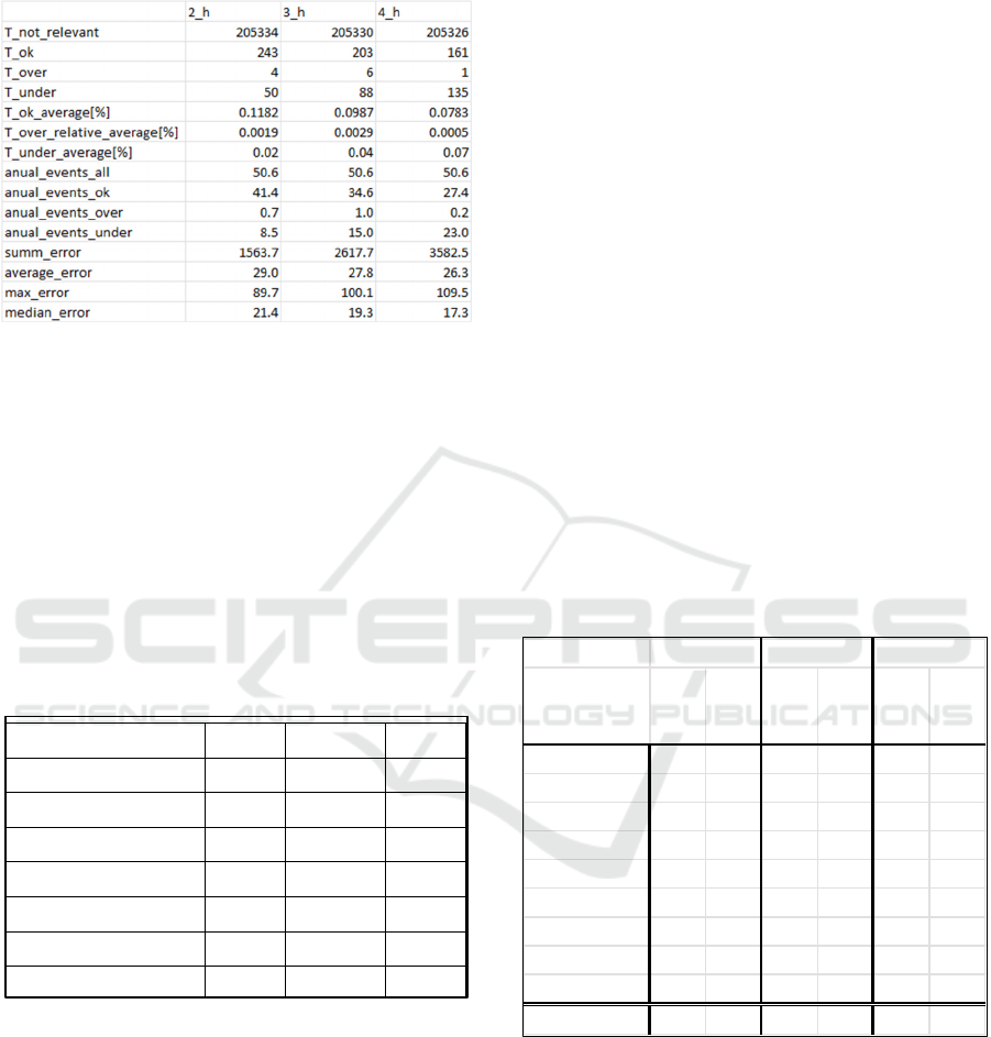
Table 4: Simple architecture LSTM-neuronal network

event-focused framework.

7.2 Evaluation of Simple LSTM

As mentioned before, the initial goal of the evaluation

framework is not only to investigate the performance

of one kind of architecture but to evaluate two or more

architectures in comparison to each other. Therefore,

a simple LSTM-ANN was prepared.

In Table 4 one can observe the apparent change of

the distribution of the time points where

measurements were overrated and underrated.

Meanwhile, the residual LSTM-ANN also has a high

number of overrated measurements during the event.

Table 5: Simple-LSTM overall metric evaluation.

The simple architecture of LSTM shows a trend

towards underrating more overrating a measurement.

With 50, 88 or 135 it has almost doubled the amount

of the underrated measurements. Furthermore, it

reduces the number of right-guessed forecasts. This

trend can be observed also in relative evaluation,

meanwhile the average error or median fails to

represent the difference. However, the overall

framework analysis in Table 5 shows that this

architecture has generally worse performance in

upper regions (NSE, IoA and modified NSE and IoA)

and awful performance in lower regions, according to

relative NSE and IoE. The interpretation of the

number is that the model makes a systematic error in

lower regions. Though the performance in higher

regions is rising, it has more errors than the residual

LSTM-ANN. This observation can be confirmed with

the event-focused evaluation in Table 4. The

performance difference during the extreme event can

be qualitatively observed in Figure 11 and Figure 12.

The observation of the overall performance of both

models can be done in Figure 10 and Figure 9.

Meanwhile, the residual ANN-model prediction

visually covers the measured level, the simple LSTM

ANN-model shows systematical overprediction in the

lower region and high underrating during extreme

events.

The Table 6 gives a comprehensive overview of

the distribution of error-chains among the models and

for the different prediction horizons. The last raw of

the table shows the average length of all chains. The

residual LSTM-ANN produces consistently slightly

shorter longest chains than the simple LSTM-ANN (9

versus 10) and also sorter chains on average (2.3:3.9;

4.1:8.1; 5.4:11).

Table 6: Distribution of chain length among models and

prediction horizons.

8 CONCLUSIONS

In this article, we presented a benchmark for machine

learning-based forecasting models. One crucial part

of the benchmark is the real-world data from the

settlement Goslar in Germany that were collected

from Harzwasserwerke GmbH for 14 years.

2h 3h 4h

BravaisPearson 0.958 0.955 0.953

(E)NSE 0.830 0.741 0.827

(d)IoA 0.955 0.924 0.947

(E)NSE_mod_J=3 0.945 0.911 0.902

(d)IoA_mod_J=3 0.992 0.985 0.981

(E)NSE_rel 0.327 ‐0.237 0.352

(

)

IoA

rel 0.822 0.636 0.800

length

simple

residual

simple

residual

simple

residual

5395108

305032

003151

001000

111121

000010

001111

010111

101010

Average length

3,9 2,3 8,2 4,1 11 5,4

2h 3h 4h

SIMULTECH 2023 - 13th International Conference on Simulation and Modeling Methodologies, Technologies and Applications

276

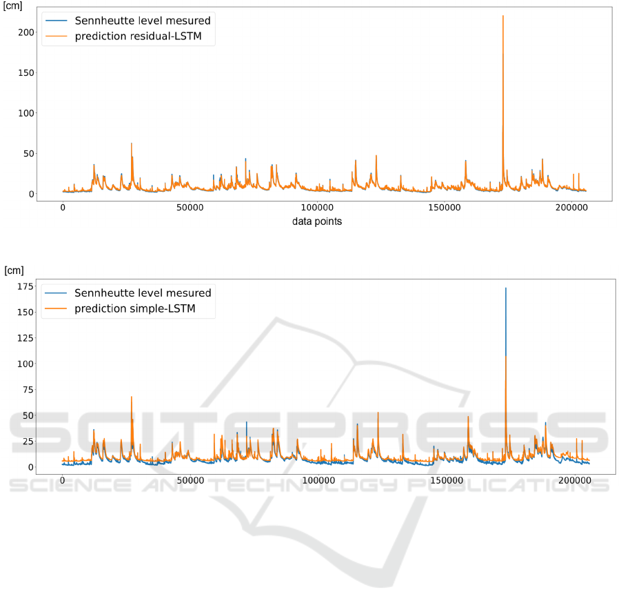
Figure 9: Overall prediction line of residual LSTM-ANN.

Figure 10: Overall prediction line of simple LSTM-ANN.

We discussed the problem that ANN are facing

during the prediction of unseen, extreme events like

floods caused by sudden rain as it happened in the

year 2017 in Goslar. The presented results of the

residual LSTM-ANN could outperform the regular

LSTM-ANN during the regular operation and the

extreme event. The discussed and presented

framework that consists of an overall evaluation

framework and event-focused evaluation framework

could prove the improvement of the used model. The

robust evaluation allows further evaluation of risks

for the city of Goslar's safety concepts. The presented

models are also a part of the actual real-time

observation system in the settlement.

Nevertheless, the benchmark gives a consolidated

and substantial challenge for machine-learning-based

models that should be applied to rare, extreme events.

The framework's flexibility also allows the evaluation

on settlements with other geological conditions.

The consolidation of the benchmark allows for

improvement in the methods of forecasting and

evaluating the constantly evolving research of

machine learning algorithms in the area of

hydrogeology.

ACKNOWLEDGEMENTS

At this point, thanks to all the people who supported

this work during the execution of the project and

preparation of this paper. Our special thanks goes to

the Harzwasserwerke GmbH for providing the data

from the measuring stations in Goslar and Bad

Harzburg and to the city of Goslar for great

collaboration and providing the local geohydrological

domain knowledge. Also our thanks to

Niedersächsischer Landesbetrieb für

Wasserwirtschaft, Küsten- und Naturschutz

(NLWKN) and Niedersächsisches Ministerium für

Umwelt, Energie und Klimaschutz for funding of the

project “Goslar - KI Hochwasserfrühwarnsystem”.

A Flood Prediction Benchmark Focused on Unknown Extreme Events

277

REFERENCES

Alfieri, L., Bisselink, B., Dottori, F., Naumann, G., Roo, A.

de, Salamon, P., Wyser, K., and Feyen, L. (2017).

“Global projections of river flood risk in a warmer

world,” Earth's Future. Vol. 5, No. 2: pp. 171–182.

Allamano, P., Claps, P., and Laio, F. (2009). “Global

warming increases flood risk in mountainous areas,”

Geophysical Research Letters. Vol. 36, No. 24.

Danso-Amoako, E., Scholz, M., Kalimeris, N., Yang, Q.,

and Shao, J. (2012). “Predicting dam failure risk for

sustainable flood retention basins: A generic case study

for the wider Greater Manchester area,” Computers,

Environment and Urban Systems. Vol. 36, No. 5: pp.

423–433.

Dtissibe, F. Y., Ari, A. A. A., Titouna, C., Thiare, O., and

Gueroui, A. M. (2020). “Flood forecasting based on an

artificial neural network scheme,” Natural Hazards.

Vol. 104, No. 2: pp. 1211–1237.

Goymann, P., Herrling, D., and Rausch, A. (2019). “Flood

Prediction through Artificial Neural Networks: A case

study in Goslar, Lower Saxony,” in ADAPTIVE 2019:

The Eleventh International Conference on Adaptive

and Self-Adaptive Systems and Applications : May 5-

9, 2019, Venice, Italy, N. Abchiche-Mimouni (ed.),

Wilmington, DE, USA: IARIA, pp. 56–62.

Hettiarachchi, P., Hall, M. J., and Minns, A. W. (2005).

“The extrapolation of artificial neural networks for the

modelling of rainfall—runoff relationships,” Journal of

Hydroinformatics. Vol. 7, No. 4: pp. 291–296.

Jimeno-Sáez, P., Senent-Aparicio, J., Pérez-Sánchez, J.,

Pulido-Velazquez, D., and Cecilia, J. (2017).

“Estimation of Instantaneous Peak Flow Using

Machine-Learning Models and Empirical Formula in

Peninsular Spain,” Water. Vol. 9, No. 5: p. 347.

Kim, S., Matsumi, Y., Pan, S., and Mase, H. (2016). “A

real-time forecast model using artificial neural network

for after-runner storm surges on the Tottori coast,

Japan,” Ocean Engineering. Vol. 122, pp. 44–53.

Krause, P., Boyle, D. P., and Bäse, F. (2005). “Comparison

of different efficiency criteria for hydrological model

assessment,” Advances in Geosciences. Vol. 5, pp. 89–

97.

Minns, A. W., and Hall, M. J. (1996). “Artificial neural

networks as rainfall-runoff models,” Hydrological

Sciences Journal. Vol. 41, No. 3: pp. 399–417.

Mosavi, A., Ozturk, P., and Chau, K. (2018). “Flood

Prediction Using Machine Learning Models: Literature

Review,” Water. Vol. 10, No. 11: p. 1536.

Mulualem, G. M., and Liou, Y.-A. (2020). “Application of

Artificial Neural Networks in Forecasting a

Standardized Precipitation Evapotranspiration Index

for the Upper Blue Nile Basin,” Water. Vol. 12, No. 3:

p. 643.

Pektas, A. O., and Cigizoglu, H. K. (2017). “Investigating

the extrapolation performance of neural network

models in suspended sediment data,” Hydrological

Sciences Journal. Vol. 62, No. 10: pp. 1694–1703.

Riad, S., Mania, J., Bouchaou, L., and Najjar, Y. (2004).

“Rainfall-runoff model usingan artificial neural

network approach,” Mathematical and Computer

Modelling. Vol. 40, 7-8: pp. 839–846.

Shamseldin, A. Y. (2010). “Artificial neural network model

for river flow forecasting in a developing country,”

Journal of Hydroinformatics. Vol. 12, No. 1: pp. 22–35.

Xu, K., Zhang, M., Li, J., Du S, S., Kawarabayashi, K., and

Jegelka, S. (2020). How Neural Networks Extrapolate:

From Feedforward to Graph Neural Networks.

SIMULTECH 2023 - 13th International Conference on Simulation and Modeling Methodologies, Technologies and Applications

278