On the Effectiveness of Re-Identiﬁcation Attacks and Local Differential

Privacy-Based Solutions for Smart Meter Data

Zeynep Sila Kaya and M. Emre Gursoy

Department of Computer Engineering, Koc¸ University, Turkey

Keywords:

Smart Meter, Energy Consumption, Privacy, Differential Privacy, Re-Identiﬁcation Attacks.

Abstract:

Smart meters are increasing the ability to collect, store and share households’ energy consumption data. On

the other hand, the availability of such data raises novel privacy concerns. Although the data can be de-

identiﬁed or pseudonymized, a critical question remains: How unique are households’ energy consumptions,

and is it possible to re-identify households based on partial or imperfect knowledge of their consumption? In

this paper, we aim to answer this question, and make two main contributions. First, we develop an adversary

model in which an adversary who observes a pseudonymized dataset and knows a limited number of con-

sumption readings from a target household aims to infer which record in the dataset corresponds to the target.

We characterize the adversary’s knowledge by two parameters: number of known readings and precision of

readings. Using experiments conducted on three real-world datasets, we demonstrate that the adversary can

indeed achieve high inference rates. Second, we propose a local differential privacy (LDP) based solution

for protecting the privacy of energy consumption data. We evaluate the impact of our LDP solution on three

datasets using two utility metrics, three LDP protocols, and various parameter settings. Results show that our

solution can attain high accuracy and low estimation error under strong privacy guarantees.

1 INTRODUCTION

Conventional electricity meters are nowadays being

replaced by smart meters which can record and trans-

mit energy consumption data to consumers and util-

ity providers. This adoption of smart meters is in-

creasing the amount of energy consumption data that

is available to be collected, stored, analyzed, and

shared. On the other hand, such availability of en-

ergy consumption data raises novel privacy risks and

concerns. Although attempts are made to de-identify

or pseudonymize consumption data, a critical ques-

tion remains: How unique are households’ energy

consumption data, and therefore, is it possible to re-

identify households based on partial and/or imperfect

knowledge of their energy consumption?

In this paper, we aim to answer this question by

constructing a realistic adversary model and empiri-

cally measuring the adversary’s success rate on real-

world energy consumption datasets. We consider

an adversary who observes a pseudonymized energy

consumption dataset, and furthermore, knows a lim-

ited number of (consumption, month) pairs of a target

household. The goal of the adversary is to infer which

record in the pseudonymized dataset corresponds to

the target household. To increase ﬂexibility, we al-

low the adversary to know ℓ (consumption, month)

pairs from the target household (we vary ℓ between

1 and 5), and we allow the adversary’s knowledge to

be precise (such as “exactly 915 kWh consumption”)

or imprecise (such as “consumption is between 900-

1000 kWh”). The number of pairs is controlled by

parameter ℓ and the degree of precision is controlled

by parameter s.

We use three real-world datasets from London and

Australia and two metrics to quantify the adversary’s

success rate: Uniqueness Ratio (UR) and Average

Anonymity Degree (AAD). UR measures what per-

centage of households in the dataset are under risk of

being uniquely identiﬁed. AAD measures the aver-

age degree of anonymity (similar to the notion of k-

anonymity) with respect to the adversary’s knowledge

characterized by ℓ and s. When adversary’s knowl-

edge is precise, results show that UR ≥ 80% as soon

as ℓ = 2. In addition, UR ≃ 100% when ℓ ≥ 3. Simi-

larly, AAD values are low (e.g., households are only 3

or 4-anonymous), which shows that re-identiﬁcation

and de-anonymization are indeed serious risks, and

psuedonymization may not be sufﬁciently effective

for privacy protection. In order to achieve reasonably

Kaya, Z. and Gursoy, M.

On the Effectiveness of Re-Identiﬁcation Attacks and Local Differential Privacy-Based Solutions for Smart Meter Data.

DOI: 10.5220/0012083300003555

In Proceedings of the 20th International Conference on Security and Cryptography (SECRYPT 2023), pages 111-122

ISBN: 978-989-758-666-8; ISSN: 2184-7711

 2023 by SCITEPRESS – Science and Technology Publications, Lda. Under CC license (CC BY-NC-ND 4.0)

111

strong privacy protection, precision needs to be heav-

ily reduced, e.g., s ≥ 2. However, such reduction in

precision (e.g., through generalization) would come

at a heavy cost of utility.

Motivated by this problem, we then explore a local

differential privacy (LDP) based approach for privacy

protection. We propose a solution in which: (i) each

household bucketizes their consumption reading, (ii)

buckets are perturbed to achieve LDP using popular

protocols such as GRR, RAPPOR or OUE, (iii) per-

turbed buckets are sent to the data collector, and (iv)

the data collector performs estimation to recover con-

sumption statistics pertaining to the general popula-

tion. In this solution, the data collector only observes

perturbed outputs of LDP protocols, not the house-

holds’ true consumption readings. The lack of a truth-

ful energy consumption dataset prevents our afore-

mentioned attack in the ﬁrst place.

We experimentally measure the impact of our pro-

posed LDP solution on three real-world datasets us-

ing various ε privacy parameters, various bucket range

sizes R, three LDP protocols (GRR, RAPPOR, OUE),

and two utility metrics (TCE and CHE) to quantify

LDP estimation error. Results show that the three pro-

tocols agree in terms of optimal R values. Further-

more, our solution is able to attain high accuracy and

low estimation error under reasonably strong privacy

guarantees (e.g., ε = 1).

The rest of the paper is organized as follows. We

review related work in Section 2. We present our ad-

versary model and experimental results with our ad-

versary model in Sections 3 and 4, respectively. We

present our solution for applying LDP to energy con-

sumption data and experimentally evaluate it in Sec-

tion 5. Finally, Section 6 concludes the paper.

2 RELATED WORK

Considering more and more data is becoming avail-

able nowadays, re-identiﬁcation and de-anonymiza-

tion attacks continue to be prominent privacy

threats. The possibility of re-identiﬁcation and de-

anonymization attacks have been shown in various

domains. The seminal work of (Sweeney, 2000)

showed that 87% of the US population can be iden-

tiﬁed using a combination of zip code, gender, and

date of birth. It is also possible to recover spe-

ciﬁc individuals’ health records by linking voter reg-

istration records with health insurance data (Ohm,

2009). The work of (Benitez and Malin, 2010) pro-

vides a set of approaches for estimating the like-

lihood of de-identifying information in the context

of data sharing policies associated with the HIPAA

privacy rule. They deﬁned two metrics and es-

timated the risk of a speciﬁc re-identiﬁcation at-

tack. In (Emam et al., 2013), a new model for es-

timating re-identiﬁcation risk was developed and ap-

plied to Canada’s post-marketing adverse drug event

database. Locations and location trace data are also

susceptible to de-anonymization and re-identiﬁcation

attacks. In (de Montjoye et al., 2013), it was shown

that human location traces are highly unique, and as

few as four low-resolution location points are enough

to uniquely identify 95% of individuals within a pop-

ulation of half million. In (Yin et al., 2015), re-

identiﬁcation risks of mobile phone users in China

were examined, and a quantitative relationship be-

tween re-identiﬁcation risk and data utility for aggre-

gate mobility analysis was studied.

Similar to these data types, smart meter and en-

ergy consumption data can also contain various pri-

vacy risks (McDaniel and McLaughlin, 2009), such as

inferring which appliances are running (Eibl and En-

gel, 2014), predicting occupancy and holidays (Tang

et al., 2015; Kleiminger et al., 2015; Eibl et al., 2019),

and determining household characteristics as well as

energy consumption proﬁles, even relating to socio-

economic status (Beckel et al., 2013; Beckel et al.,

2014; Anderson et al., 2017; Cz

any et al., 2021).

Among different privacy risks, closer to our work

are attacks that focus on de-anonymization and re-

identiﬁcation. In (Buchmann et al., 2012), it was

shown that households can be re-identiﬁed using sim-

ple statistical measures, and even simple means are

sufﬁcient to re-identify 68% of the records. Higher

de-pseudonymization rates were achieved in later

studies such as (Tudor et al., 2015) and (Cleemput

et al., 2018). In a very recent work by (Radovanovic

et al., 2022), the authors demonstrated that even if

consumption data are anonymized, it is possible to

identify a household with high accuracy by utilizing

weekly consumption.

The prevalence of privacy risks associated with

smart meters and energy consumption data has led to

growing interest in engineering new privacy solutions

based on obfuscation and/or perturbation (Pal et al.,

2018; Khwaja et al., 2020). Towards this aim, in this

paper, we consider the application of Local Differen-

tial Privacy (LDP). LDP has recently gained signiﬁ-

cant attention from academia and industry (Cormode

et al., 2018; Gursoy et al., 2022), but its applications

to smart meters and smart grid have been relatively

few. In (Ou et al., 2020), a singular spectrum analysis-

based LDP method has been proposed to prevent in-

ference of household appliances. (Gai et al., 2022)

developed a data aggregation scheme with LDP using

randomized response. In (Parker et al., 2021), a new

SECRYPT 2023 - 20th International Conference on Security and Cryptography

112

Table 1: Sample energy consumption data (in kWh) from 4

households and across 4 months.

id 01/2021 02/2021 03/2021 04/2021

1 1108 915 1013 972

2 802 712 788 793

3 278 241 267 312

4 551 462 495 479

variant of differential privacy called spectral DP was

proposed, motivated by applications with unbounded

time-series data such as smart meter data. A literature

review covering the applications of different forms of

differential privacy (not just LDP) was conducted in

(Marks et al., 2021).

3 ADVERSARY MODEL

3.1 Problem Setting and Notation

Consider a monthly energy consumption dataset as

shown in Table 1. Each row corresponds to a different

household and each column corresponds to a different

month. The dataset shows how much energy (in kWh)

was consumed by each household in each month, e.g.,

measured by a smart meter. For example, household

1 consumed 972 kWh in April 2021. The dataset

is completely pseudonymized, i.e., random IDs are

assigned to each row (determined arbitrarily) which

aims to hide the identity of the corresponding house-

holds. Note that each row can be viewed as one time

series corresponding to the monthly energy consump-

tion of one household.

We denote the full dataset by D. Without loss of

generality, we write D = {T

,...,T

} to denote that

D contains n households, where T

denotes the energy

consumption time series of the i’th household. We

write T

[ j] to refer to the consumption amount of T

the j’th month. All time series in D have equal length,

i.e., |T

| = |T

| = ... = |T

3.2 Adversary Formulation

We consider an adversary A who observes the

pseudonymized dataset D, and furthermore, knows a

limited number of (consumption, month) pairs from

a certain household h. We denote this knowledge of

the adversary by K = {(c

),(c

),...} where

is to the consumption amount (in kWh) and m

is the corresponding month. For example, K =

{(802,01/2021),(712,02/2021)} means that the ad-

versary knows the household h has consumed 802

kWh in January 2021 and 712 kWh in February 2021.

The adversary is assumed to formulate such knowl-

edge K through third-party resources or accessing

meter readings in the physical world (e.g., observing

h’s electricity bill).

Given D and K , the goal of A is to infer which

time series in D corresponds to the household h. If the

adversary is successful in uniquely identifying h from

the dataset, then the adversary learns the remaining

energy consumption readings of h. Continuing from

the example in the previous paragraph, in Table 1,

there is only one household which satisﬁes the knowl-

edge K = {(802,01/2021),(712,02/2021)}. Then,

the adversary learns that id = 2 corresponds to house-

hold h; furthermore, the consumption readings of h

for March 2021 is 788 kWh and for April 2021 it is

793 kWh. Note that such an inference can be quite

sensitive in practice. For example, if a household

consumes much lower energy in certain months com-

pared to the rest of the months (e.g., in July-August

the consumption is much lower) then this may indi-

cate that the residents go on holiday or the household

is unoccupied during these months.

The success of the adversary relies heavily on the

amount of knowledge K available. We introduce two

parameters for characterizing K : length ℓ and preci-

sion s.

Length ℓ denotes how many (consumption,

month) pairs are known by the adversary, i.e., ℓ = |K |.

When ℓ is small, e.g., ℓ = 1, it is more likely that

there are multiple households in D which ﬁt the ad-

versary’s knowledge. For example, in a dataset with

thousands of households, there can be multiple house-

holds which have the same consumption reading for

January 2021. On the other hand, as the value of ℓ

increases, we expect the uniqueness of households to

also increase.

Precision s: We account for cases in which the adver-

sary’s knowledge K may be imprecise. For example,

instead of knowing that h’s consumption in January

2021 is 802, the adversary may know that consump-

tion is within the range [800, 900) without knowing

the exact amount. The reason for the imprecision in

K could be due to an inexact observation, as well as a

potential privacy protection method (i.e., through gen-

eralization or masking).

In our work, we account for the imprecision us-

ing parameter s. The smallest possible value of s is

s = 0, which means that A knows the exact integer

consumption amount, e.g., consumption in January

2021 is 802. When s = 1, one least signiﬁcant digit

of the consumption amount is not known by the ad-

versary. For example, instead of knowing the con-

sumption amount is 802, the adversary knows that it

is 80*, i.e., between [800, 810). When s = 2, two least

signiﬁcant digits are not known, e.g., the adversary’s

On the Effectiveness of Re-Identiﬁcation Attacks and Local Differential Privacy-Based Solutions for Smart Meter Data

113

Figure 1: Monthly consumption of ﬁve households.

knowledge is equal to 8** which corresponds to the

range [800, 900). In general, s is equal to the number

of least signiﬁcant digits that are not known by the

adversary (or are masked).

We visualize the impact of s using sample con-

sumption data in Figure 1. When s is smaller, unique-

ness of households increases. For example, when

s = 2 and K consists of the knowledge [300, 400),

there are two households which ﬁt this criteria. When

s = 3 and K consists of the knowledge [0, 1000),

there are ﬁve households which ﬁt this criteria. In

general, as s increases, we expect households’ unique-

ness to decrease.

3.3 Measurement Metrics

Given an adversary who has D and K , we would like

to measure: (i) What percentage (ratio) of households

can the adversary uniquely identify? (ii) How anony-

mous are the households? To answer these two ques-

tions, we deﬁne the following two metrics.

Uniqueness Ratio (UR): We say that K uniquely

identiﬁes a household in D if and only if there exists

exactly one T

∈ D such that:

∀(c

) ∈ K : T

] = c

In other words, given K , the adversary will be able

to uniquely identify T

in D since there does not exist

any other time series which ﬁts the conditions in K .

Given D, ℓ and s, we generate all possible com-

binations of knowledge that an adversary may have

which satisfy the ℓ and s parameters. Let K denote

this set of all possible combinations. Note that K is

potentially a very large set, e.g., for a single house-

hold and ℓ = 1, there are |T | different entries in K,

one for each month. Then, the Uniqueness Ratio of

dataset D is deﬁned as:

UR =

# of K ∈ K that uniquely identiﬁes

a household in D

|K|

By deﬁnition, the metric takes values between [0, 1].

Values closer to 0 imply better privacy for households

(lower uniqueness).

Average Anonymity Degree (AAD): We say that T

is k-anonymous with respect to K if and only if there

exist k − 1 other time series S ⊂ D such that:

∀T ∈ S, ∀(c

) ∈ K : T [m

] = T

] = c

In other words, T

appears indistinguishable from

|S| = k − 1 other time series to an adversary who has

knowledge K . Note that this is an adaptation of the

well-known notion of k-anonymity (Sweeney, 2002;

Samarati, 2001; Fung et al., 2010). Instead of requir-

ing T

to be indistinguishable from k − 1 other time

series in terms of all monthly consumption readings,

our formulation requires T

to be indistinguishable in

terms of only the adversary’s knowledge K .

Let us deﬁne a function Φ which takes as input T

D and K and outputs the anonymity degree of T

in D

with respect to K . That is: Φ(T

,D,K ) = k. Then,

we generate all possible combinations of knowledge

K similar to UR. Finally, Average Anonymity Degree

(AAD) is formally deﬁned as:

AAD =

∑

K ∈K

∑

i=1

Φ(T

,D,K )

|D| × |K|

Intuitively, AAD measures the anonymity degree

of all time series in D in terms of all possible adver-

sarial knowledge K ∈ K. Then, their average is com-

puted to arrive at AAD. In the best case of privacy, all

time series are indistinguishable from one another in

terms of all K . In this case, AAD becomes equal to

|D|. In the worst case, where all time series are only

1-anonymous, AAD becomes equal to 1.

4 EXPERIMENT RESULTS AND

DISCUSSION

4.1 Experiment Setup and Datasets

We experimented with three real-world energy con-

sumption datasets to measure the effectiveness of the

aforementioned adversary model using the metrics

given in Section 3.3. In our experiments, ℓ is var-

ied between 1 and 5, and s is varied between 0 and 3.

These parameters were chosen as such because of the

SECRYPT 2023 - 20th International Conference on Security and Cryptography

114

following reasons: For s, the consumption readings in

our datasets rarely went over 10.000; therefore all val-

ues of s ≥ 3 would have had the same practical impact

as s = 3. Hence, maximum s was determined as 3. For

ℓ, we experimentally observed that ℓ = 5 is sufﬁcient

to cause either perfect or near-perfect uniqueness in

many cases; thus, increasing it further would not have

changed our results and ﬁndings.

Our three datasets come from two sources: The

ﬁrst dataset is from the London Datastore, whereas

the second and third datasets are from Ausgrid, an

electricity distribution company in Australia. The

datasets are explained in more detail below.

London: The London Datastore is a platform es-

tablished by the Greater London Authority to share

data relating to the city of London. We extracted

the Smart Meter Energy Consumption Data in Lon-

don Households from (Datastore, 2023), which con-

tains energy consumption readings for 5567 London

households that took part in Low Carbon London

project. Data collection occurred from November

2011 to February 2014; however, since many mea-

surements in the years 2011 and 2014 as well as the

ﬁrst six months of 2012 were missing, we focused on

the 18-month time period from July 2012 to Decem-

ber 2013. We also removed households whose read-

ings contained null values, resulting in 4369 remain-

ing households. Finally, to ensure consistency with

our adversary model and remaining datasets, we ag-

gregated the data in (Datastore, 2023) into monthly

consumptions per household.

Solar: This dataset was provided by Ausgrid,

an electricity distribution company in Australia. We

downloaded the Solar Home Monthly Data from

(Ausgrid, 2023), which contains electricity consump-

tion data for 2657 solar households with rooftop solar

systems installed in their houses. The data is provided

for the time period between January 2007 and Decem-

ber 2014. After inspecting the Solar dataset, we ob-

served 589 null (missing) values. We used backward

interpolation to eliminate them.

Non-solar: Similar to the Solar dataset, the Non-

solar dataset was also provided by Ausgrid. It can be

accessed through the same URL. The dataset contains

monthly energy consumption of 4064 households that

had never installed a solar system. The Non-solar

dataset also covers the time period between January

2007 and December 2014.

4.2 UR and AAD Results

In this section, we present Uniqueness Ratio (UR) and

Average Anonymity Degree (AAD) results under dif-

ferent s and ℓ parameters. We use the plots in Figure

2 to show how UR results change according to s and

ℓ. Interestingly, we observed very similar trends in

all three datasets. First, as expected, as we increase

s from 0 to 3, UR values decrease. A signiﬁcant re-

duction is obtained even when s is changed from 0

to 1. Furthermore, UR values are very close to 0

when s ≥ 2, yielding good privacy for households.

This shows that reducing the precision of the adver-

sary’s knowledge, e.g., through generalization, is a

possible solution against the adversary model consid-

ered in this paper. Second, we observe that as we

increase ℓ from 1 to 5, UR values increase substan-

tially. Although UR values are lower than 20% when

ℓ = 1, they jump to ≥ 80% when ℓ = 2 (assuming

s = 0 in both cases). In other words, the fact that

the attacker knows two consumption readings of the

victim household rather than one reading increases

the probability of uniquely identifying that household

roughly 4 times. In general, UR values are alarm-

ingly high when ℓ ≥ 3 and s ≤ 1. In many cases,

almost all households become uniquely identiﬁable

(UR ≃ 100%). In order to prevent identiﬁcation and

keep UR low, substantial reduction in precision must

be present (i.e., s = 2 or 3).

We use the heatmaps in Figure 3 to report the

changes in AAD values according to the s and ℓ

parameters. In general, across all three datasets,

anonymity levels decrease as ℓ increases and s de-

creases. Note that AAD values on the Solar dataset

are relatively lower than the other datasets, but this

is because the Solar dataset is smaller than the oth-

ers. Interestingly, AAD values are quite high when

s ≥ 2, meaning that households can remain reason-

ably anonymous even when the adversary knows ℓ =

5 readings. On the other hand, a large difference is

observed between s = 1 and s = 2. When s = 1, as

long as ℓ ̸= 1, AADs are low (such as 1, 2, 4, 7)

which means that households become almost unique

in terms of their consumptions. When s = 0, low

AADs are observed across all ℓ, i.e., all AADs con-

verge to 1.

Combining the results presented in this section,

in addition to conﬁrming our expectations regarding

the AAD and UR impacts of ℓ and s, we empirically

observe that: (i) precise knowledge of consumption

readings (s = 0) can indeed cause high risk of unique

identiﬁcation for households, (ii) knowing more than

ℓ = 1 consumption readings greatly increases the risk

of identiﬁcation and greatly decreases the degree of

anonymity, and (iii) high amount of imprecision, such

as s = 2 or 3, must be introduced in order to prevent

adversarial inference effectively.

On the Effectiveness of Re-Identiﬁcation Attacks and Local Differential Privacy-Based Solutions for Smart Meter Data

115

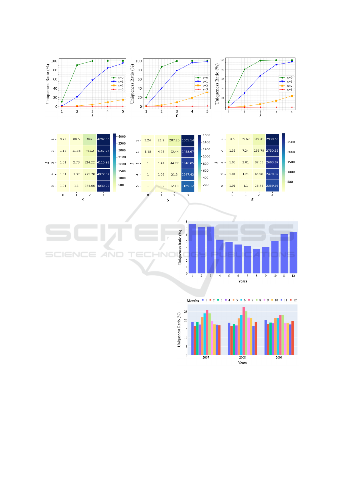
Figure 2: UR results on London, Solar, and Non-solar datasets respectively.

Figure 3: AAD results on London, Solar, and Non-solar datasets respectively.

4.3 Impact of Seasonality

Next, in order to examine the impact of seasonality,

we measure how UR results change from month to

month in a calendar year. To do so, we construct

knowledge K for each month separately and compute

UR values in each month. The results are given in

Figures 4, 5 and 6. On the London dataset, we per-

form this experiment only in year 2013, since 2013

is the only full year of data available. Three different

years (2007, 2008, 2009) are considered for the Solar

and Non-solar datasets. In all results, ℓ = 1 and s = 0

are used.

An interesting observation from the London

dataset is that UR results are lower between

months June-September, whereas they are consider-

ably higher between months January-March (e.g., 4%

UR vs 8% UR). In other words, uniqueness drops in

summer months whereas it rises in the winter months.

A similar behavior is observed on Solar and Non-solar

datasets, but since these datasets are from Australia,

winter months are close to June-August whereas sum-

mer months are closer to January-March. Never-

theless, UR results are considerably higher in win-

ter months compared to summer months. Further-

more, across different years and different datasets

(2007 to 2009), this observation holds consistently.

Thus, we ﬁnd that uniqueness of households may in-

deed be impacted by seasons and weather conditions.

Households typically consume higher energy in cold

Figure 4: Seasonality on London dataset (year: 2013).

Figure 5: Seasonality on Solar dataset.

weather, and since households have different char-

acteristics, they are likely to be reﬂected by the in-

creased uniqueness ratios during winter.

SECRYPT 2023 - 20th International Conference on Security and Cryptography

116

Figure 6: Seasonality on Non-solar dataset.

5 APPLICATION OF LOCAL

DIFFERENTIAL PRIVACY

(LDP)

Various approaches can be developed to address

privacy risks concerning energy consumption data.

Our results in the previous section showed that

generalization-based methods constitute one possi-

ble option to reduce UR and AAD; however, large

amount of generalization is necessary for them to be

effective (e.g., s = 2). Another option is the use of dif-

ferential privacy (DP) such that the full dataset is D is

collected by the data collector in plaintext; yet, only

a noisy access interface is provided to researchers

and/or adversaries. However, the shortcomings of this

approach are twofold: (i) it remains susceptible to

side channel attacks, and (ii) it assumes that house-

holds inherently trust the data collector to hold their

data in plaintext. Instead, in this paper we advocate

for the use of local differential privacy (LDP) which

recently emerged as a state-of-the-art notion for pri-

vacy protection.

5.1 LDP and LDP Protocols

In LDP, there exist several households (clients) and a

data collector (server). To ensure LDP, each client’s

true consumption is encoded and perturbed by a ran-

domized algorithm Ψ on the client side, and the per-

turbed output is sent to the data collector. Thus, the

collected dataset D consists of perturbed readings,

and households’ true consumption readings are never

revealed in D. Consequently, LDP can be used in

scenarios where the data collector is untrusted by the

households. Formally, LDP is deﬁned as follows.

Deﬁnition 1 (ε-LDP). A randomized algorithm Ψ

satisﬁes ε-local differential privacy (ε-LDP), where

ε > 0, if and only if for any two inputs v

in uni-

verse U, it holds that:

∀y ∈ Range(Ψ) :

Pr[Ψ(v

) = y]

Pr[Ψ(v

) = y]

≤ e

(1)

where Range(Ψ) denotes the set of all possible out-

puts of Ψ.

After collecting perturbed readings from many

clients, the data collector needs to perform estima-

tion to recover statistics pertaining to the client popu-

lation. For value v ∈ U, let C(v) denote the true count

of v, i.e., number of times v is actually observed in

the population. Let

C(v) denote the estimated count

of v, i.e., the count estimated by the server after LDP.

The difference between C(v) and

C(v) is called the

estimation error. Several LDP protocols were devel-

oped in the literature for minimizing estimation error

under various settings. In this paper, we will use three

popular LDP protocols: GRR, RAPPOR, and OUE.

Generalized Randomized Response (GRR): is a

generalization of the randomized response survey

technique introduced in (Warner, 1965) to support

non-binary U and arbitrary ε. Denoting by v the

client’s true value, the perturbation algorithm Ψ

GRR

perturbs v and outputs y ∈ U with probability:

Pr[Ψ

GRR

(v) = y] =

(

p =

+|U|−1

if y = v

q =

+|U|−1

if y ̸= v

(2)

where |U| denotes the size of the universe. This sat-

isﬁes ε-LDP since

= e

. The client sends y to the

server.

On the server side, upon receiving perturbed out-

puts from all clients, to perform estimation for some

value v

∗

∈ U the server ﬁrst ﬁrst ﬁnds

C(v

∗

): total

number of clients who reported v

∗

as their perturbed

output. Then, estimate

C(v

∗

) is computed as:

C(v

∗

) =

C(v

∗

) − |L| · q

p − q

(3)

where |L| denotes the number of clients in the popu-

lation.

RAPPOR: was originally developed by Google and

implemented in Chrome (Erlingsson et al., 2014;

Fanti et al., 2016). While the original version of RAP-

POR relies on Bloom ﬁlters for string encoding, in

this paper we leverage a variant of RAPPOR which

uses unary encoding, similar to (Wang et al., 2017;

Gursoy et al., 2019).

Client initializes a bitvector B with length |U|.

The client sets B[v] = 1 and for all remaining posi-

tions j ̸= v, those positions are set as: B[ j] = 0. Then,

the perturbation step of RAPPOR takes as input B and

outputs a perturbed vector B

′

. Perturbation algorithm

On the Effectiveness of Re-Identiﬁcation Attacks and Local Differential Privacy-Based Solutions for Smart Meter Data

117

RAP

considers each bit in B one by one, and either

keeps or ﬂips the bit with probabilities:

∀

i∈[1,|U|]

: Pr[B

′

[i] = 1] =

(

ε/2

if B[i] = 1

ε/2

if B[i] = 0

(4)

The client sends perturbed bitvector B

′

to the server.

The server receives perturbed bitvectors B

′

from

all clients in the population. To perform estimation

for value v

∗

, Sup(v

∗

) is computed as the total number

of received bitvectors that satisfy: B

′

∗

] = 1. Then,

the estimate

C(v

∗

) is computed as:

C(v

∗

) =

Sup(v

∗

) + |L| · (α −1)

2α − 1

(5)

where α is the bit keeping probability: α =

ε/2

Optimized Unary Encoding (OUE): has the same

encoding phase as RAPPOR with unary encoding, but

its bit keeping and ﬂipping probabilities are different.

It treats the 0 and 1 bits asymmetrically to improve

accuracy of server-side estimation (Wang et al., 2017;

Jia and Gong, 2019).

Client initializes bitvector B with length |U| such

that B[v] = 1, and for all remaining positions j ̸= v,

B[ j] = 0. Perturbation algorithm Ψ

OUE

takes as input

B and produces perturbed bitvector B

′

such that:

∀

i∈[1,|U|]

: Pr[B

′

[i] = 1] =

(

if B[i] = 1

if B[i] = 0

(6)

The client sends perturbed bitvector B

′

to the server.

The server receives perturbed bitvectors B

′

from

all clients in the population. To perform estimation

for value v

∗

, Sup(v

∗

) is computed as the total number

of received bitvectors that satisfy: B

′

∗

] = 1. Then,

the estimate

C(v

∗

) is computed as:

C(v

∗

) =

2 ·



+ 1) · Sup(v

∗

) − |L|



− 1

(7)

5.2 Enforcing LDP on Energy

Consumption Data

GRR, RAPPOR and OUE protocols assume a discrete

universe U and perform perturbation within this dis-

crete universe. Since households’ energy consump-

tion readings are typically numeric and continuous,

these protocols are not directly applicable to energy

consumption data. A straightforward solution for this

problem would be to discretize each numeric con-

sumption reading by rounding it to the nearest integer.

However, this is also not a desirable solution, since it

causes U to be extremely large. To exemplify, recall

that the real-world datasets from Section 4 contained

Algorithm 1: Our application of LDP.

Input : Household population L , privacy

parameter ε, bucket range size R,

number of buckets N, month j

Output: Estimates

C(·) for month j

/* Client-side perturbation */

1 U ← {0, 1, 2, ...,N − 1}

2 for i ∈ L do

3 v ← T

[ j]//R

4 x ← Perturb v using LDP protocol with

parameters ε and U // use Eqn 2,

4 or 6 for GRR, RAPPOR or OUE

5 Send x to the server

6 end

/* Server-side estimation */

7 for v

∗

∈ [0, N − 1] do

C(v

∗

) ← Estimate using LDP protocol

with parameters ε and U // use Eqn

3, 5 or 7

9 end

10 return

C(v

∗

) for all v

∗

4369, 2657 and 4064 households respectively, mean-

ing that the number of households is in the order of

1000s. Considering that minimum consumption read-

ing is typically 0 and maximum consumption reading

can be quite large (e.g., 10000s or more), our U would

be in the order of 10000s which is a magnitude larger

than the number of households. This would cause

the resulting statistics (i.e., number of households per

unique reading) to be extremely sparse, which nega-

tively impacts estimation utility. Additionally, large

U also causes efﬁciency problems because the com-

putational complexities of many protocols such as

GRR, RAPPOR and OUE are at least linear in terms

of U, i.e., they are Ω(|U|).

Motivated by the above problems, we propose the

following solution for applying LDP to energy con-

sumption readings via bucketization. Given the range

size (bucket size) R and the number of buckets N,

we ﬁrst construct buckets: [0,R), [R,2R), [2R,3R),

..., [NR − R,NR]. When household i would like to

perturb his/her consumption reading at month j, de-

noted by T

[ j], the household ﬁrst computes his/her

true value as v = T

[ j]//R, where // denotes integer

division. This way, the household’s consumption is

assigned to one of the N buckets, and the true value v

of the household becomes the number of that bucket.

Considering there are N buckets, the universe U is

now limited to: U = {0,1, ...,N −1}. After the house-

hold’s true value v is determined and U is known as

above, v can be fed into one of GRR, RAPPOR or

OUE protocols, and the perturbed output can be ob-

SECRYPT 2023 - 20th International Conference on Security and Cryptography

118

tained. The household sends the perturbed output to

the data collector. After collecting perturbed outputs

from all households, the data collector (server) per-

forms estimation to ﬁnd how many households are es-

timated to have consumption readings in each bucket.

The overall process is summarized in Algorithm

1. As explained above, ﬁrst the universe of buckets

U ← {0,1,2,...,N − 1} is initialized on line 1 of the

algorithm. Then, between lines 3-6, each household

bucketizes his/her true value (line 3) and then perturbs

it using an LDP protocol (line 4) such as GRR, RAP-

POR or OUE. Outcome of the perturbation is sent

to the server (line 5). After the server receives per-

turbed outputs from all households, the server per-

forms estimation (lines 7-9). Since values have been

bucketized, the estimation of the server needs to be

performed bucket-by-bucket. Thus, for each bucket

(line 7), the estimation algorithm of the correspond-

ing LDP protocol is used (line 8) such as GRR, RAP-

POR or OUE. Results of the estimations are produced

as the output of Algorithm 1 (line 10).

5.3 Quantifying Estimation Error

Due to the perturbation of LDP, the estimates recov-

ered by Algorithm 1 will be imperfect, i.e., they will

contain error. We propose two error metrics to mea-

sure estimation error: Consumption Histogram Error

(CHE) and Total Consumption Error (TCE).

Consumption Histogram Error (CHE): Algorithm

1 recovers noisy LDP estimates

C(v

∗

) for v

∗

∈ [0,N −

1], which can be viewed as a histogram of number of

households that have value v

∗

= 0,1,...,N −1. In con-

trast, let C(v

∗

) denote the true number of households

that have value v

∗

which would have been learned if

all households’ consumption readings were observed

in plaintext (i.e., no privacy protection). CHE is com-

puted as the average difference between

C(v

∗

) and

C(v

∗

), i.e.:

CHE =

N−1

∑

∗

C(v

∗

) −C(v

∗

Total Consumption Error (TCE): The total energy

consumption of all households in the population is

important to preserve, since it is important for demand

and capacity planning in a city or an electricity grid.

Let ϕ be the true total energy consumption in the cur-

rent month, which would have been computed if all

households’ consumption readings were observed in

plaintext. On the other hand, using the output of Al-

gorithm 1, the expected total energy consumption un-

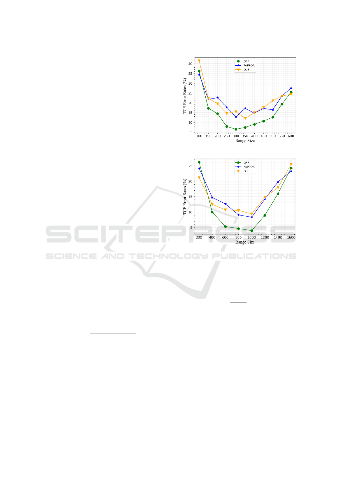
Figure 7: TCE results on London dataset (ε = 1).

Figure 8: TCE results on Non-solar dataset (ε = 1).

der LDP, denoted by

ϕ, can be computed as:

ϕ =

N−1

∑

∗

C(v

∗

) ×



∗

R +



Then, TCE is computed as:

TCE =

ϕ − ϕ|

× 100%

Multiplication by 100% is performed to turn TCE into

a percentage and thereby increase interpretability.

5.4 LDP Experiment Results

In order to measure the potential real-world impact of

our LDP solution via simulation, we perform experi-

ments using the same datasets and setup from Section

4. We focus on the impacts of two parameters: pri-

vacy budget ε and range size R. We measure error

amounts using TCE and CHE metrics. We perform

experiments separately for different months in each

dataset, compute the values of TCE and CHE metrics,

and then take their average across all months.

In Figures 7 and 8, we ﬁx ε = 1 and vary R, in

order to analyze the impact of varying R on TCE. On

On the Effectiveness of Re-Identiﬁcation Attacks and Local Differential Privacy-Based Solutions for Smart Meter Data

119

Table 2: TCE results on London (left), Non-solar (mid), Solar (right) datasets.

ε GRR RAPPOR OUE

0.1 95.64 135.12 171.72

0.5 16.05 27.99 27.24

1 6.59 15.55 13.24

2 2.80 5.02 5.32

4 1.00 3.46 2.71

6 0.63 1.69 1.77

ε GRR RAPPOR OUE

0.1 81.93 108.77 105.50

0.5 11.52 20.54 19.07

1 4.04 10.29 10.12

2 1.63 5.57 4.27

4 0.88 2.37 2.18

6 0.71 1.38 1.64

ε GRR RAPPOR OUE

0.1 53.46 84.39 80.45

0.5 8.29 19.39 19.42

1 3.86 9.22 9.78

2 1.38 4.67 4.61

4 0.66 2.01 2.61

6 0.45 1.27 2.02

Table 3: CHE results on London (left), Non-solar (mid), Solar (right) datasets.

ε GRR RAPPOR OUE

0.1 664.32 701.64 806.13

0.5 142.19 170.14 164.30

1 67.86 95.65 89.50

2 28.36 39.76 45.54

4 8.38 21.73 23.09

6 3.05 11.69 20.64

ε GRR RAPPOR OUE

0.1 695.97 769.16 779.02

0.5 139.16 167.92 161.46

1 55.83 86.07 87.68

2 26.12 43.90 43.48

4 8.69 19.75 26.68

6 3.17 11.32 20.19

ε GRR RAPPOR OUE

0.1 532.10 539.31 602.10

0.5 108.97 139.72 150.01

1 50.65 73.46 70.67

2 20.84 35.68 36.92

4 6.72 16.15 21.75

6 2.36 9.20 18.28

both datasets and all three LDP protocols, the results

show a U-shaped curve trend. In other words, in Fig-

ure 7, starting from R = 100 and gradually increas-

ing R, we observe that TCE results decrease until R

is between the 250-350 range, and afterwards TCE

results start to increase as R is further increased to

R > 350. Similarly, in Figure 8, starting from R = 200

and gradually increasing R, TCE results decrease un-

til R is between 600-800, and afterwards TCE starts

to increase as R is further increased. These ﬁgures

and observations yield three key insights. First, our

proposed solution using bucketization is indeed more

effective than simply rounding consumption readings

to the nearest integer and then applying LDP. Round-

ing to the nearest integer is equivalent to setting R = 1,

which, according to these results, would be expected

to yield much higher TCE. Second, GRR, RAPPOR

and OUE protocols all agree in the U-shaped curve

trend, and they approach minimal error amounts for

similar R. Due to their consistency, it is possible to

choose R in a protocol-agnostic manner, and an R

value that yields good results for one protocol is likely

to yield good results also for other protocols. Third,

assuming the use of a good R value, it is possible to

estimate total consumptions with TCE ≤ 5% or 10%

even with a reasonably strict privacy budget of ε = 1.

This shows that our proposed solution is feasible and

can yield good utility in practice.

In Tables 2 and 3, we ﬁx R and vary ε, in order

to analyze the impact of varying ε on TCE and CHE.

In this experiment, we chose near-optimal values of

R, that is: R = 300 for London dataset, R = 800 for

Non-solar dataset, and R = 500 for Solar dataset. Re-

sults with the TCE metric are reported in Table 2 and

results with the CHE metric are reported in Table 3.

We observe that the GRR protocol has lower error

in terms of both TCE and CHE compared to RAP-

POR and OUE across many ε settings. ε = 0.1 is the

strictest privacy budget we use, and indeed, we ob-

serve that errors are quite high in this case. As we

increase ε from 0.1 to 0.5, errors are substantially re-

duced. As we increase ε further to 1, 2, 4 and 6, errors

are further reduced, although at a lower speed com-

pared to the reduction from 0.1 to 0.5. When ε ≥ 4,

TCE values are ≤ 1% and CHE values contain single

digit, negligible errors (in case of GRR).

6 CONCLUSION

In this paper, we made mainly two contributions at

the intersection of privacy and energy consumption

data. First, we proposed an adversary model in which

an adversary observes a pseudonymized energy con-

sumption dataset and knows a limited number of con-

sumption readings of a target household. The knowl-

edge of the adversary is characterized by a length pa-

rameter ℓ and a precision parameter s. Using three

real-world datasets and UR and AAD metrics, we ex-

perimentally showed the effectiveness of such an ad-

versary’s re-identiﬁcation ability. Second, we pro-

posed a LDP and bucketization-based solution for

protecting the privacy of households’ consumption

readings. We measured the estimation error caused

by our solution under various settings and parameter

choices using CHE and TCE metrics. Results showed

that our solution is able to achieve low estimation er-

ror under reasonably strong privacy guarantees such

as ε = 1.

There are several directions for future work. First,

we plan to study the results of the UR and AAD met-

rics after our LDP and bucketization-based solution

from Section 5 is applied to the data. Second, we plan

to integrate several additional LDP protocols to our

SECRYPT 2023 - 20th International Conference on Security and Cryptography

120

work, which can reduce client-server communication

cost (e.g., hashing-based protocols such as BLH and

OLH) in bandwidth-constrained environments. Third,

recall from Section 5 that bucket sizes are equal for

all buckets (R). We plan to investigate the utility and

privacy impacts of uneven bucket sizes, e.g., whether

uneven bucket sizes can help improve estimation util-

ity, and whether small bucket sizes may increase the

risk of identiﬁability. Furthermore, we plan to in-

vestigate whether bucket sizes can be automatically

learned from the underlying data.

ACKNOWLEDGEMENTS

We gratefully acknowledge the support from The

Scientiﬁc and Technological Research Council of

Turkiye (TUBITAK) under project number 121E303.

REFERENCES

Anderson, B., Lin, S., Newing, A., Bahaj, A., and James, P.

(2017). Electricity consumption and household char-

acteristics: Implications for census-taking in a smart

metered future. Computers, Environment and Urban

Systems, 63:58–67.

Ausgrid (2023). Solar home electricity data.

https://www.ausgrid.com.au/Industry/Our-Research/

Data-to-share/Solar-home-electricity-data.

Beckel, C., Sadamori, L., and Santini, S. (2013). Auto-

matic socio-economic classiﬁcation of households us-

ing electricity consumption data. Proceedings of the

fourth international conference on Future energy sys-

tems.

Beckel, C., Sadamori, L., Staake, T., and Santini, S. (2014).

Revealing household characteristics from smart meter

data. Energy, 78:397–410.

Benitez, K. and Malin, B. (2010). Evaluating re-

identiﬁcation risks with respect to the hipaa privacy

rule. Journal of the American Medical Informatics

Association, 17:169–177.

Buchmann, E., B

ohm, K., Burghardt, T., and Kessler, S.

(2012). Re-identiﬁcation of smart meter data. Per-

sonal and Ubiquitous Computing, 17:653–662.

Cleemput, S., Mustafa, M. A., Marin, E., and Preneel, B.

(2018). De-pseudonymization of smart metering data:

Analysis and countermeasures. 2018 Global Internet

of Things Summit (GIoTS).

Cormode, G., Jha, S., Kulkarni, T., Li, N., Srivastava, D.,

and Wang, T. (2018). Privacy at scale: Local differen-

tial privacy in practice. In Proceedings of the 2018

International Conference on Management of Data,

pages 1655–1658. ACM.

any, L., V

amos, V., Horv

ath, M., Szalay, Z., Mota-

Babiloni, A., Deme-B

elaﬁ, Z., and Csoknyai, T.

(2021). Development of electricity consumption pro-

ﬁles of residential buildings based on smart meter data

clustering. Energy and Buildings, 252:111376.

Datastore, L. (2023). Smartmeter energy

consumption data in london house-

holds. https://data.london.gov.uk/dataset/

smartmeter-energy-use-data-in-london-households.

de Montjoye, Y.-A., Hidalgo, C. A., Verleysen, M., and

Blondel, V. D. (2013). Unique in the crowd: The pri-

vacy bounds of human mobility. Scientiﬁc Reports,

Eibl, G., Burkhart, S., and Engel, D. (2019). Insights into

unsupervised holiday detection from low-resolution

smart metering data. In International Conference on

Information Systems Security and Privacy (ICISSP),

pages 281–302. Springer.

Eibl, G. and Engel, D. (2014). Inﬂuence of data granularity

on smart meter privacy. IEEE Transactions on Smart

Grid, 6(2):930–939.

Emam, E., Dankar, F. K., Neisa, A., and Jonker, E. (2013).

Evaluating the risk of patient re-identiﬁcation from

adverse drug event reports. BMC Medical Informat-

ics and Decision Making, 13.

Erlingsson,

U., Pihur, V., and Korolova, A. (2014). Rappor:

Randomized aggregatable privacy-preserving ordinal

response. In Proceedings of the 2014 ACM SIGSAC

Conference on Computer and Communications Secu-

rity, pages 1054–1067. ACM.

Fanti, G., Pihur, V., and Erlingsson,

U. (2016). Building a

rappor with the unknown: Privacy-preserving learning

of associations and data dictionaries. Proceedings on

Privacy Enhancing Technologies, 2016(3):41–61.

Fung, B. C., Wang, K., Chen, R., and Yu, P. S. (2010).

Privacy-preserving data publishing: A survey of re-

cent developments. ACM Computing Surveys (CSUR),

42(4):1–53.

Gai, N., Xue, K., Zhu, B., Yang, J., Liu, J., and He, D.

(2022). An efﬁcient data aggregation scheme with lo-

cal differential privacy in smart grid. Digital Commu-

nications and Networks, 8(3):333–342.

Gursoy, M. E., Liu, L., Chow, K.-H., Truex, S., and Wei,

W. (2022). An adversarial approach to protocol anal-

ysis and selection in local differential privacy. IEEE

Transactions on Information Forensics and Security,

17:1785–1799.

Gursoy, M. E., Tamersoy, A., Truex, S., Wei, W., and

Liu, L. (2019). Secure and utility-aware data collec-

tion with condensed local differential privacy. IEEE

Transactions on Dependable and Secure Computing,

18(5):2365–2378.

Jia, J. and Gong, N. Z. (2019). Calibrate: Frequency es-

timation and heavy hitter identiﬁcation with local dif-

ferential privacy via incorporating prior knowledge. In

IEEE International Conference on Computer Commu-

nications (INFOCOM), pages 2008–2016. IEEE.

Khwaja, A. S., Anpalagan, A., Naeem, M., and Venkatesh,

B. (2020). Smart meter data obfuscation using cor-

related noise. IEEE Internet of Things Journal,

7(8):7250–7264.

On the Effectiveness of Re-Identiﬁcation Attacks and Local Differential Privacy-Based Solutions for Smart Meter Data

121

Kleiminger, W., Beckel, C., and Santini, S. (2015). House-

hold occupancy monitoring using electricity meters.

In Proceedings of the 2015 ACM International Joint

Conference on Pervasive and Ubiquitous Computing,

pages 975–986.

Marks, J., Montano, B., Chong, J., Raavi, M., Islam, R.,

Cerny, T., and Shin, D. (2021). Differential privacy

applied to smart meters: a mapping study. In Proceed-

ings of the 36th Annual ACM Symposium on Applied

Computing, pages 761–770.

McDaniel, P. and McLaughlin, S. (2009). Security and pri-

vacy challenges in the smart grid. IEEE Security &

Privacy Magazine, 7:75–77.

Ohm, P. (2009). Broken promises of privacy: Responding

to the surprising failure of anonymization. UCLA Law

Review, 57:1701.

Ou, L., Qin, Z., Liao, S., Li, T., and Zhang, D. (2020). Sin-

gular spectrum analysis for local differential privacy

of classiﬁcations in the smart grid. IEEE Internet of

Things Journal, 7(6):5246–5255.

Pal, R., Hui, P., and Prasanna, V. (2018). Privacy engineer-

ing for the smart micro-grid. IEEE Transactions on

Knowledge and Data Engineering, 31(5):965–980.

Parker, K., Hale, M., and Barooah, P. (2021). Spectral

differential privacy: Application to smart meter data.

IEEE Internet of Things Journal, 9(7):4987–4996.

Radovanovic, D., Unterweger, A., Eibl, G., Engel, D., and

Reichl, J. (2022). How unique is weekly smart meter

data? Energy Informatics, 5.

Samarati, P. (2001). Protecting respondents identities in mi-

crodata release. IEEE Transactions on Knowledge and

Data Engineering, 13(6):1010–1027.

Sweeney, L. (2000). Simple demographics often iden-

tify people uniquely. Health (San Francisco),

671(2000):1–34.

Sweeney, L. (2002). k-anonymity: A model for protecting

privacy. International Journal of Uncertainty, Fuzzi-

ness and Knowledge-Based Systems, 10(05):557–570.

Tang, G., Wu, K., Lei, J., and Xiao, W. (2015). The meter

tells you are at home! non-intrusive occupancy detec-

tion via load curve data. In 2015 IEEE International

Conference on Smart Grid Communications (Smart-

GridComm), pages 897–902. IEEE.

Tudor, V., Almgren, M., and Papatriantaﬁlou, M. (2015). A

study on data de-pseudonymization in the smart grid.

Proceedings of the Eighth European Workshop on Sys-

tem Security.

Wang, T., Blocki, J., Li, N., and Jha, S. (2017). Locally

differentially private protocols for frequency estima-

tion. In Proc. of the 26th USENIX Security Sympo-

sium, pages 729–745.

Warner, S. L. (1965). Randomized response: A survey tech-

nique for eliminating evasive answer bias. Journal of

the American Statistical Association, 60(309):63–69.

Yin, L., Wang, Q., Shaw, S.-L., Fang, Z., Hu, J., Tao, Y., and

Wang, W. (2015). Re-identiﬁcation risk versus data

utility for aggregated mobility research using mobile

phone location data. PLOS ONE, 10:e0140589.

SECRYPT 2023 - 20th International Conference on Security and Cryptography

122