Interaction-Based Task Group Scheduling for a Scalable and Real-Time

Self-Driving Simulation

Akihito Kohiga

, Kei Hiroi

, Takumi Kataoka

, Sho Fukaya

and Yoichi Shinoda

Information Science Japan Advanced Institute of Science and Technology, Ishikawa, Japan

Disaster Prevention Research Institute Kyoto University, Kyoto, Japan

Applied Information Engineering Suwa University of Science, Nagano, Japan

shinoda@jaist.ac.jp

Keywords:

Virtual Machine, Vehicular Simulation, Real-Time Scheduling.

Abstract:

We developed a self-driving test environment based on Virtual Machine (VM) technology. Our test envi-

ronment enables us to test multiple types of self-driving Artiﬁcial Intelligences (AIs) in one simulation and

import their self-driving software to an actual car without modiﬁcation. Our test environment divides a map

into several segments and assigns a physical machine to each segment. If a vehicle crosses a border, the VM

that embodies the vehicle is moved to another physical machine. However, VM movement causes a load

imbalance on the physical machines. We suggest a novel approach to assign high-priority processing to a

group of vehicles. The group of vehicles consists of one target vehicle that we would like to test and other

vehicles that may interact with the target vehicle. We create such a group by identifying interactions using a ”

pre-simulation”. Our approach reduced the processing time of the jobs created by the self-driving AIs by more

than 90 percent under an ideal condition . This result indicates that our approach contributes the real-time

processing when the CPU was in an overcommitted state.

1 INTRODUCTION

Many serious accidents occur during trials of self-

driving systems. The website (Sel, 2023) lists serious

incidents during self-driving. AI takes a long time to

learn the appropriate behavior with many scenarios.

To prevent an actual driver in a self-driving vehicle

from having a serious accident, many precise com-

puter simulations should be performed before a ﬁeld

trial. A computer simulation can create many scenar-

ios that are too difﬁcult and dangerous to run in real-

ity; thus, it reduces serious accidents before trials on

public roads.

Many self-driving vehicle simulators exist, such

as CARLA (Dosovitskiy et al., 2017), Udacity Self-

Driving Car Simulation (uda, 2017), and Microsoft’s

AirSim (air, 2017). These self-driving vehicle sim-

ulators have several problems related to ”ﬂexibility.”

CARLA, Udacity Self-Driving Car Simulation, and

AirSim were developed as monolithic applications;

hence, essentially, they cannot be modiﬁed as paral-

lel applications on a cloud computer. Consequently,

they lack scalability. They have ”ﬁxed” APIs to ac-

cess data inside the applications. When we require

additional data that their APIs do not provide, we can-

not acquire such data. if we requested additional APIs

to the developers, it would take a long time to imple-

ment.

It would be ideal if we could run many scenarios

with many types of simulated cars and export self-

driving AI from a simulation environment to a real ve-

hicle without any modiﬁcations. To accomplish these

requirements, the self-driving simulator would clearly

not be as described in previous studies. Self-driving

simulators require more ﬂexibility to achieve scalabil-

ity and improve their ability to access data.

Our objective is to develop a ﬂexible and scalable

test environment for self-driving AI. Figure 1 shows

an overview of the suggested environment. Our simu-

lation environment consists of VMs, a driving simula-

tor, a 3D map simulator, and simulation middleware.

In the ﬁgure, a driving simulator and 3D map sim-

ulator are connected to virtual devices in a VM via

simulation middleware and share information. The

3D simulator creates a virtual space and continuously

sends pictures as a camera view to a virtual camera

device on a VM. The driving simulator receives the

rotation angle from the steering wheel and the ac-

Kohiga, A., Hiroi, K., Kataoka, T., Fukaya, S. and Shinoda, Y.

Interaction-Based Task Group Scheduling for a Scalable and Real-Time Self-Driving Simulation.

DOI: 10.5220/0012083800003546

In Proceedings of the 13th International Conference on Simulation and Modeling Methodologies, Technologies and Applications (SIMULTECH 2023), pages 287-294

ISBN: 978-989-758-668-2; ISSN: 2184-2841

 2023 by SCITEPRESS – Science and Technology Publications, Lda. Under CC license (CC BY-NC-ND 4.0)

287

celeration value from a virtual steering wheel (and

virtual acceleration pedal and brake) in a VM. The

driving simulator calculates its direction and veloc-

ity from the rotation angle and acceleration value re-

ceived, and sends them to the 3D map simulator to up-

date the vehicle’s location. Developers of self-driving

AI can execute any task they develop in a VM, their

own AI, and any libraries and runtimes. In Figure 1,

ROS (Quigley et al., 2009) is used at the runtime en-

vironment in a VM.

Figure 1: VM-based simulation environment.

The data transaction in the suggested type of self-

driving simulation has ”geographical locality”. The

geographical locality of a data transaction means that

the data transaction often occurs between objects that

are geographically close to each other in a simulation.

In the case of a trafﬁc simulation that has two self-

driving vehicles that are about to encounter each other

at a blind corner, they would perform a data transac-

tion via a wireless ad hoc network to avoid a trafﬁc

accident. At the point of computation, VMs that are

geographically close to each other in the simulation

should be placed on a same physical machine to elim-

inate the data transaction over a physical network in a

data center, otherwise network congestion would oc-

cur.

Figure 2 shows the VM deployment mechanism in

our environment(Kohiga and Shinoda, 2020). The left

side of the ﬁgure describes a trafﬁc simulation, and

the right side describes a simulation cloud. In this

example, the simulation map is separated into sev-

eral segments and, at least one physical machine is

assigned to each segment of the map. A VM repre-

sents a self-driving vehicle.

For example, in Figure 2, there are two vehicles in

Area #1 and the Physical Machine 1(PM1) is assigned

to Area#1. Two VMs are executed on PM1. If a self-

driving vehicle moves over the boundary of the two

areas, the VM representing this self-driving vehicle

moves to another physical machine. In the case of

Figure 2, when a self-driving vehicle in Area#1 moves

to Area#2, the VM that represents its vehicle on PM1

also moves to PM2.

(vehicle #1)

Area#1 Area#2

Area#3

Area#4

map

PM3

(Area #3)

PM1

(Area #1)

(vehicle #1)

PM4

(Area #4)

PM2

(Area#2)

(train #1)

(vehicle #3)

(vehicle #1)

(vehicle #4)

(“PM” stands for “Physical Machine”)

Figure 2: Division of the simulation map into several areas

and assignment of them to each physical machine.

Our simulation environment has more scalability

and ﬂexibility, compared with the previous works.

2 CHALLENGES

The biggest problem in our simulation environment is

how to maintain real-time processing when there are

several spontaneous increases of VMs in one segment

described in Figure 2.

The simulation clock synchronization of all simu-

lation objects is the most important task in a loosely

coupled simulation environment. All simulation ob-

jects must maintain a simulation clock that is syn-

chronized with the others, otherwise the simulation

would lose credibility. In the case of a trafﬁc simu-

lation, a car crash that should occur does not occur

because of the clock skew. Several techniques exist

for the synchronization of the clock in an agent-based

simulation. The most obvious technique is to have

“global virtual time” (GVT) (Fujimoto, 2001). GVT

is a clock system that is shared by all processing ob-

jects that appear in a simulation. Once GVT is set, all

processes should obey this time.

There is a case in which the lack of CPUs spon-

taneously occurs during a simulation in our environ-

ment. Figure 3 shows a typical case in which a part

of the simulation in a VM is delayed. The left side

of the ﬁgure describes a simulation map and vehicles.

The right side of the ﬁgure describes task scheduling

with a timeline. We explained the deployment mech-

anism of our simulation environment in Figure 2. As

the simulation proceeds, the number of vehicles in an

area varies. At a certain moment, a number of vehi-

cles exceeds a number of CPUs assigned in the seg-

ment. There are four vehicles on the left-hand side

of the ﬁgure; hence, four VMs should be executed on

the physical machine assigned to this segment. This

physical machine has only two CPUs; hence, the ex-

ecution of these VMs are delayed because of the lack

of a CPU. In this case, the time lapse is twice as fast

as that for the clock inside the VMs (when the real

clock is T = 2, the VMs execute task A and task B at

SIMULTECH 2023 - 13th International Conference on Simulation and Modeling Methodologies, Technologies and Applications

288

Area

CPU

(t=0)

Time

T=0 T=1

T=2

(t=0)

(t=1)

Figure 3: A inﬂux of vehicles in one segment induces the

lack of CPUs in our simulation environment.

t = 1).

The simulation delay in one segment propagates

to all VMs in our simulation environment if they have

a time synchronization mechanism like GVT. Conse-

quently, the end of a simulation gets behind because

of spontaneous increase of VMs on only one segment.

Therefore, we would like to suggest how to maintain

real-time processing when there are several sponta-

neous increases of VMs in a segment.

3 RELATED WORKS

High Level Architecture(HLA)(Dahmann, 1997) is

the most famous middleware that federates indepen-

dent simulators in one simulation. Compared with our

simulation environment, HLA processes a federated

simulation with smaller time, but forces each sim-

ulator to embed APIs to access the HLA functions.

We are considering how to utilize the functionality

of HLA (ex. time synchronization, data exchange) in

virtual machine mechanism and it would be good step

for next federation.

Many studies also have been conducted that are re-

lated to task scheduling for cloud computing, which is

essentially used to reduce the turn around time (TAT)

of a request from outside a data center. Its tech-

nique is based on how many requests are assigned

to each computer with a certain criterion (request

priority, energy aware, high CPU utilization, etc.).

Task scheduling-related studies were categorized by

Mathew et al. (Mathew et al., 2014). The unique

feature of our simulation environment is the sponta-

neous movement of VMs. According to the explana-

tion in Figure 2, if a self-driving vehicle moves over

the boundary of the area, the VM that represents the

self-driving vehicle also moves to another physical

machine. This deployment mechanism uses the “geo-

graphical locality” of the data transaction between the

VMs and simulators, but the spontaneous movement

of VMs occurs. A load balancing mechanism cannot

control such spontaneous movement. This feature oc-

curs a load imbalancing and has not been studied in

previous work in this ﬁeld.

4 INTERACTION-BASED TASK

GROUP SCHEDULING

4.1 Basic Concept

A feasible solution is to choose a minimum set of

VMs to which high priority is assigned to avoid the

lack of resources. We deﬁne a minimum set of VMs

as the VMs that consists of one target VM and the

others which interact with the target VM. A developer

who is creating a self-driving AI running on the target

VM must test whether the self-driving AI smoothly

negotiates with other self-driving AIs when they en-

counter each other in a critical scenario (e.g., negotia-

tion at a blind corner). In such tests, if we choose a set

of VMs that interact with the target self-driving AI,

we can ignore synchronization with the other VMs.

Figure 4 shows the image of vehicles grouped in

a simulation. There are ﬁve vehicles (VehicleA to

VehicleE) in the ﬁgure and they have a direction to

move in (depicted by an arrow). VehicleA is mov-

ing down a road and VehicleB is moving up the same

road. Finally, they pass each other somewhere on this

road. If they have cameras for object recognition,

then these cameras must capture the opposite vehi-

cle (the camera on VehicleA captures VehicleB, and

vice versa). Similar to VehicleA and VehicleB, Vehi-

cleC, VehicleD, and VehicleE pass each other on the

right-hand side of the area; hence, they are captured

by each other’s cameras. We refer to VehicleA and

VehicleB as “GroupA” and VehicleC, VehicleD, and

VehicleE as “GroupB.” In the ﬁgure, vehicles that be-

long to GroupA have never encountered the vehicles

that belong to GroupB; therefore, we can set differ-

ent priorities for each group. If we have to observe

the behavior of VehicleA, we can set a high priority

for vehicles that belong to GroupA. By contrast, we

must ignore the behavior of vehicles that belong to

GroupB.

GroupA GroupB

Figure 4: Basic concept is to compose the vehicles which

interact with each other in a group and observe one group’s

behavior.

Interaction-Based Task Group Scheduling for a Scalable and Real-Time Self-Driving Simulation

289

Figure 5 indicates the relationship between the

elapsed time and the vehicle’s position. The rectangle

on the left-hand side indicates the positions of two ve-

hicles for a certain time (t = 0) and the rectangle on

the right-hand side indicates the positions of two ve-

hicles for another time (t = 1). The two vehicles are

about to interact somewhere on a road at t = 0 and

then they move in their own directions at t = 1. Un-

til the two vehicles pass each other, they belong to

the same group and we must assign the same priority

to them. However, after they have interacted and are

moving in different directions, they are independent

from each other and we no longer assign the same

priority to them. To acquire the relation between the

elapsed time and the vehicle’s position, we must pre-

dict the interactions before we run a self-driving sim-

ulation.

Interact (t=0) Not Interact (t=1)

Figure 5: Two vehicles are not in one group after they pass

each other.

”Interaction” refers to a scenario in which a vehi-

cle is visible to another vehicle’s sensor. Many types

of sensors exist and common feature of these sensors

is that they have an ”effective range”. For example,

a camera has a range of dozens of meters that shapes

sector in front and LiDAR has a range of several me-

ters that shapes circular. If a vehicle moves into the

range of the sensor, self-driving AI recognizes it as

an object and then makes some decisions Therefore,

we deﬁne interaction as a scenario in which a vehicle

moves into the effective range of a sensor and inter-

acts with a self-driving AI’s decision. Our simulation

environment must obtain the effective range of sen-

sors to create the aforementioned groups.

4.2 Overview of Our Approach

4.2.1 Requirement

We mentioned that our suggested mechanism requires

a starting point and route information from each VM

before the simulation starts. This is a precondition

for interaction-based priority settings. In this paper,

we do not discuss which interface is appropriate be-

cause it is simply an implementation matter and out

of scope for our study. We only have to acquire start-

ing points and route information from each VM using

some type of method. To acquire the starting points

and route information from each VM requires, at a

minimum, more than one interface between the VMs

and simulation management middleware.

4.2.2 Control Flow

The basic concept of our solution is to change the in-

teraction information in a simulation to the priority

settings on each VM. We divide this basic concept

into the following four parts.

1. (Trafﬁc Simulation) acquires the current location

and route information from each VM, executes a

trafﬁc simulation with them, and acquires the re-

sult ﬁle, which records the position of each ve-

hicle and the direction sorted by time. We could

regard this sequence as a ”pre-simulation”.

2. (Interaction Search) searches interactions from

the result ﬁle created in the previous step. Inter-

action search creates a time series interaction list,

which consists of a set of clocks , the two vehi-

cles’ IDs, and an interaction symbol (unilateral or

mutual).

3. (Grouping) creates priority information for each

VM from the interaction information. Grouping

sequence creates a group of vehicles. The group

consists of ”a target vehicle” and the other vehi-

cles that interact with the target vehicle. In this

sequence, we must select one vehicle as the target

vehicle.

4. (Priority Control) sends priority settings to every

virtual clock in accordance with the high-priority

group information.

The above four parts are shown in Figure 6. These

sequences are processed on the simulation middle-

ware. The grouping sequence creates ﬁles that include

priority information for each VM, which is the list of

priority settings for every clock from the simulation

start time. Priority Control sends a priority setting to

every clock that corresponds to the same clock in the

priority ﬁle.

In contrast to the periodic process for Priority

Control, the Trafﬁc Simulation in the simulation mid-

dleware gathers starting points and route information

from each VM once before the simulation starts. If

some VMs change their route, the simulation middle-

ware must execute Interaction Search and Grouping

again because the route change affects the interaction

information between vehicles.

SIMULTECH 2023 - 13th International Conference on Simulation and Modeling Methodologies, Technologies and Applications

290

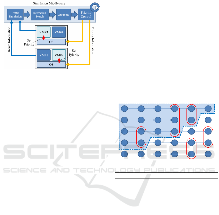
Figure 6: Priority Control ﬂow in our simulation environ-

ment.

4.3 Interaction Search

Interaction Search searches the interactions in the

simulation. As we mentioned, we must choose one

vehicle as the target vehicle and then search the ve-

hicles that interact with the target vehicle. Finally,

Interaction Search generates the time series interac-

tion list, which consists of a set of clocks, the two

vehicles’ IDs, and their distance between them. For

an effectiveness experiment in this study, we use the

SUMO (Krajzewicz et al., 2002) trafﬁc simulator to

obtain the starting points and route information in-

stead of acquiring them from each vehicle. SUMO

has a program that randomly generates any number of

vehicles in a simulation, including the starting points

and route information. We also use SUMO as the traf-

ﬁc simulation for the Trafﬁc Simulation on the simu-

lation middleware. We assume that the current posi-

tion and route information can be acquired from each

VM. Route information can also be acquired from

each VM. The self-driving AI must set the destina-

tion and route information before departure; hence,

this information must exist whenever we run the “pre-

simulation”.

4.4 Grouping

Grouping creates priority information for each VM

from interaction information. Our mechanism creates

a group of vehicles that consists of ”a target vehicle”

and other vehicles that interact with the target vehicle.

As we mentioned in the deﬁnition of interaction in

Figure 5, two vehicles interact somewhere on a road

at t = 0 and then move in their own directions at t = 1.

These two vehicles are included in one group at t = 0,

but they are not in the same group at t = 1. Therefore,

the number of vehicles in the group is greatest at the

start time of the simulation and then decreases as time

progresses.

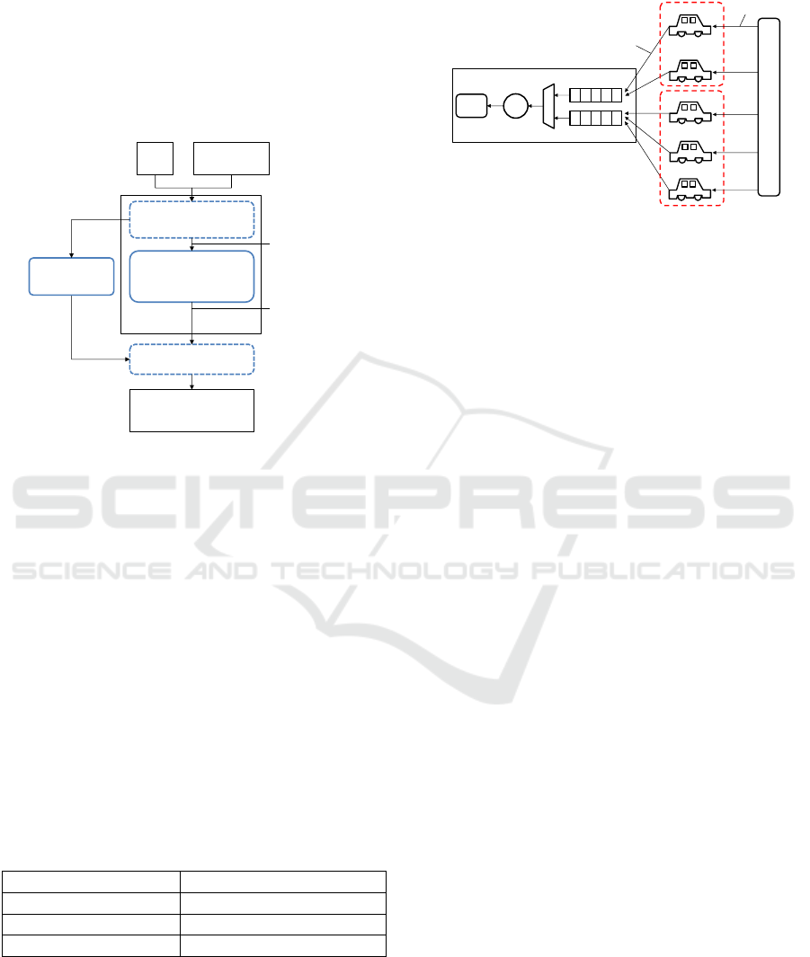
Figure 7 shows a time sequence that describes the

Grouping process. Each circle with a capital letter

represents one vehicle and the horizontal axis (from

T = 0 to T = 5) indicates the elapsed time. An arrow

in this ﬁgure represents a vehicle moving to another

place; hence, VehicleA at T = 0 has a different posi-

tion from VehicleA at T = 1. A red oval represents

an interaction and has two meanings : unilateral in-

teraction and mutual interaction. For example, Vehi-

cleC and VehicleD have two interactions at T = 1 and

T = 5, and VehicleA, VehicleB, and VehicleC have

one interaction at T = 3. A short dashed line sur-

rounds almost half of the ﬁgure, which indicates the

group that we ﬁnally want to create. The ﬁgure de-

scribes the group of VehicleA. The group of VehicleA

means ”VehicleA as a target vehicle and the other ve-

hicles that interact with VehicleA”.

T=0

T=1

T=2

T=3

T=4

T=5

Figure 7: Grouping.

Data 1: Group Data (result of Grouping).

[(’VehicleID’, clock), ...]

[(’91.0’,19.0),(’87.0’,15.0),(’99.0’,12.0),

(’15.0’,12.0),(’57.0’,11.0),(’43.0’,7.0)]

Finally, we acquire the group data described in

Data 1. A tuple consists of the vehicle ID and clock.

Clock in this data means the last clock when the high-

priority setting of its vehicle is canceled. In the case

of vehicle ID ”A” and clock ”10.0,” our simulation

middleware assigns a high priority to vehicle A” from

the starting time (normally 0.0) to ”10.0” in the simu-

lation.

5 EVALUATION

Figure 8 shows the basic sequence of the evaluation

environment. The basic sequence is composed of the

map and route information of every vehicle as in-

put, simulation middleware, the VM deployment al-

gorithm, and a cloud simulator. The simulation mid-

Interaction-Based Task Group Scheduling for a Scalable and Real-Time Self-Driving Simulation

291

dleware is also composed of a trafﬁc simulator and

other parts. We prepared the SUMO trafﬁc simulator

to generate the vehicle’s position and also prepared

the following three components: interaction search,

grouping, and priority setting . The simulation mid-

dleware created the priority setting of each vehicle

and input them into the cloud simulator. We used a

cloud simulator instead of an actual cloud to process

the job.

dƌĂĨĨŝĐƐŝŵƵůĂƚŽƌ

;^hDKͿ

• /ŶƚĞƌĂĐƚŝŽŶƐĞĂƌĐŚ

• 'ƌŽƵƉŝŶŐ

• WƌŝŽƌŝƚǇƐĞƚƚŝŶŐ

ůŽƵĚƐŝŵƵůĂƚŽƌ

;KDEdннͿ

DĂƉ

ZŽƵƚĞ

/ŶĨŽƌŵĂƚŝŽŶ

sĞŚŝĐůĞ͛ƐƉŽƐŝƚŝŽŶ

ΘĚŝƌĞĐƚŝŽŶŽŶ

ĞǀĞƌǇ ĐůŽĐŬ

WƌŝŽƌŝƚǇƐĞƚƚŝŶŐ

sDůŽĐĂƚŝŽŶŽŶ

ĞǀĞƌǇ ĐůŽĐŬ

sD ĚĞƉůŽǇ

ĂůŐŽƌŝƚŚŵ

sĞŚŝĐůĞ͛Ɛ

ƉŽƐŝƚŝŽŶŽŶ

ĞǀĞƌǇĐůŽĐŬ

^ŝŵƵůĂƚŝŽŶ

ŵŝĚĚůĞǁĂƌĞ

KƵƚƉƵƚ

;ƉƌŽĐĞƐƐŝŶŐƚŝŵĞ

ŽĨĞĂĐŚũŽďͿ

Figure 8: Basic sequence of the evaluation.

Table 1 shows the conﬁguration that we used for

the trafﬁc simulation on the simulation middleware.

The SUMO trafﬁc simulator requires a map, a starting

point and route information for each vehicle as input.

We created a grid-shaped load map and the vehicle’s

information using scripts that are part of the SUMO

simulator. Vehicles were generated in the range from

100 to a maximum of 500 vehicles at the beginning

of the simulation. We prepared two methods to create

a vehicle’s route: one based on a random walk and

another that compel the vehicles to move through a

designated place. The lesser the interaction the better

for reducing the number of vehicles that are assigned

high priority. A random walk is an ideal method to

reduce interactions. In contrast to a random walk, a

trafﬁc jam is the worst scenario at the point of reduc-

ing interactions.

Table 1: Trafﬁc simulation parameters.

map 2km square 400 junctions

number of vehicles 100 to 500

simulation time(s) 200 to 1000

route of each vehicles Random

We describe the details of the cloud simulator in

Figure 9. The cloud simulator is based on a queuing

system. A physical machine is composed of one CPU,

one sink, two queues, and one selector. The number

of physical machines also changes in accordance with

how many physical machines are used for the simula-

tion.

High Priority

Low Priority

Selector

CPU

Sink

GroupB

GroupA

Simulation Middleware

set priority

input jobs

Figure 9: Cloud simulator (OMNET++).

A vehicle receives priority information and VM

location. Priority information is a set of time and pri-

ority. When a vehicle receives a set of time and prior-

ity such as (4.0, high), the source changes the job’s

priority to high immediately and the high-priority

state is ﬁnished by the 4.0 clock. A vehicle send a

job to a high priority queue during high-priority state.

The source also receives VM location information

When a vehicle receives the new location, the vehi-

cle sends the next job to another physical machine.

5.1 Evaluation Points

We consider the following points for the evaluation

of our approach. The objective of our approach is to

create a minimum group of vehicles and assign high

priority to them to maintain real-time processing. The

smaller number of vehicles in one group is the better.

These points are the basic evaluation to observe the

feature of our mechanism.

1. measure the processing time of jobs with a ﬁxed

number of vehicles and ﬁxed duration as a fun-

damental evaluation, and then compare the two

cases: our approach assigns high priority to the

minimum group of vehicles and a normal scenario

in a priority property is not assigned;

2. measure the processing time using our approach

in the case in which the simulation time is in-

creased;

3. investigate differences in the number of interac-

tions between vehicles running with a random

walk and vehicles that stay in a trafﬁc jam

5.2 Result

5.2.1 Fundamental Evaluation

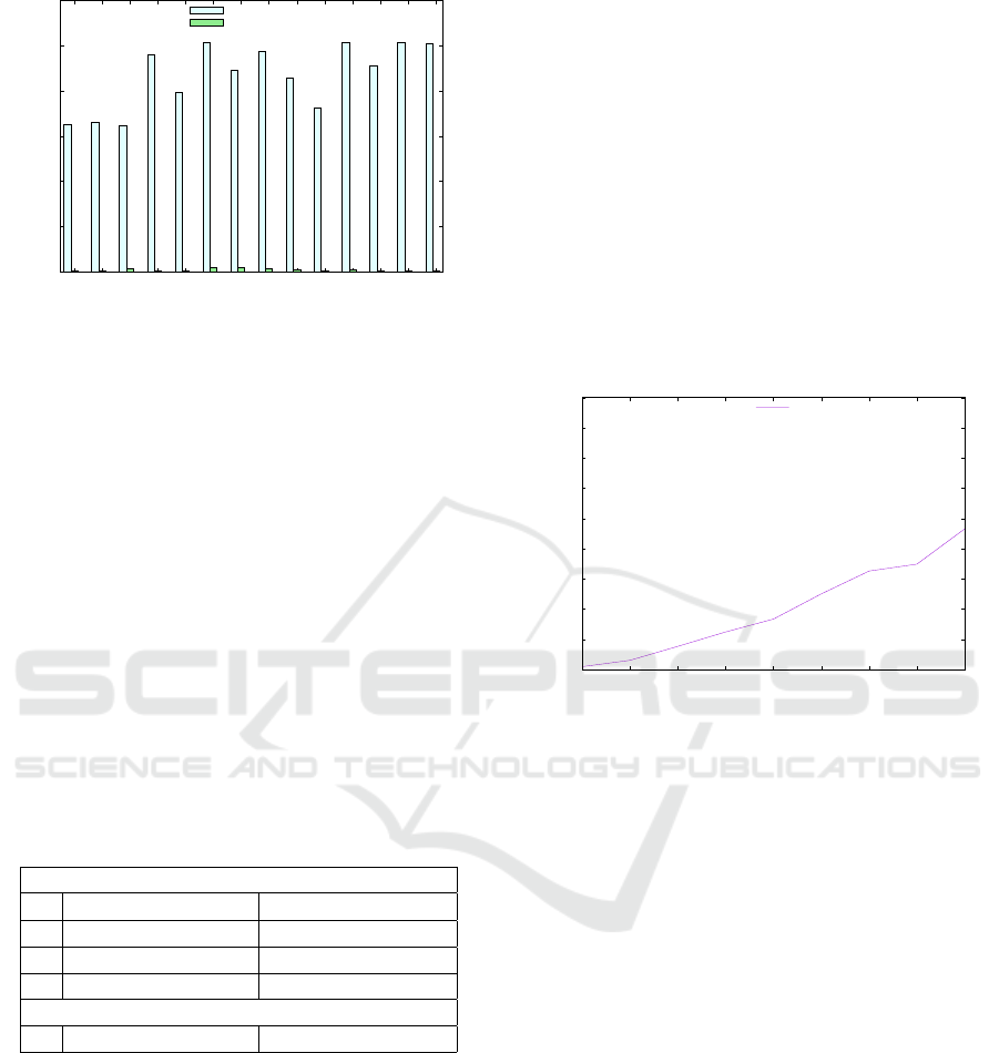
Figure 10 shows the fundamental evaluation result of

our approach. We also describe the conﬁguration of

SIMULTECH 2023 - 13th International Conference on Simulation and Modeling Methodologies, Technologies and Applications

292

100

200

300

400

500

600

0.0 33.0 20.0 11.0 85.0 55.0 75.0 77.0 88.0 23.0 50.0 7.0 30.0 67.0

processing time (ms)

Vehicle IDs

without priority

our approach

Figure 10: Fundamental evaluation of our approach.

this evaluation in Table 2.

Figure 10 shows that our approach effectively re-

duced the processing time compared with the process-

ing time without our approach. The x-axis represents

the individual vehicle IDs and the y-axis represents

the average processing time of jobs produced by each

vehicle. The best case is vehicle ID ”30.0”. The pro-

cessing time with our approach was 3.03 milliseconds

and the processing time without our approach was

507.53 milliseconds, which means that our approach

reduced the processing time by approximately 99.3

percent. The worst case was the vehicle ID ”55.0” In

this case, our approach reduced the processing time

by approximately 98 percent of the processing time

without our approach. The average processing time

with our approach was 4.703 milliseconds and that

without our approach was 432.808. Therefore, our

approach reduced the processing time by 99 percent.

Table 2: Conﬁguration of the fundamental evaluation.

Trafﬁc simulation conﬁguration

map 2km

400 junctions

number of vehicles 200

simulation time(s) 200

routes Random

physical macine conﬁguration

the number of PCs 9 nodes (4cores)

The jobs produced by vehicles took 2 milliseconds

to be processed. Therefore, if they were smoothly

processed without waiting on a queue, the ideal re-

sult of the above evaluation would be 2 milliseconds.

The average processing time with our approach was

4.703 milliseconds. This means that some jobs were

slightly stacked on a physical machine. Later, we dis-

cuss whether this delay is reasonable for the real-time

processing of a self-driving simulation.

5.2.2 Increasing the Duration of a Simulation

Figure 11 shows the relationship between the dura-

tion of a simulation and the processing time. The

conﬁguration of this evaluation is the same as that of

the fundamental evaluation. This result indicates that

our approach could not maintain real-time processing

in a simulation that had a long duration. Consider-

ing the 400-second duration in the graph, the average

processing time was approximately 50 milliseconds.

Generally, a delay is barely noticeable up to 50 mil-

liseconds and is acceptable up to 100 milliseconds if

no high demands with respect to realism are required.

Therefore, the duration of a simulation should be less

than 600 seconds for this conﬁguration.

100

150

200

250

300

350

400

450

200 300 400 500 600 700 800 900 1000

average of processing time (ms)

Duration of a simulation (s)

"result.csv" using 1:2

Figure 11: Inﬂuence on increasing the duration of the sim-

ulation.

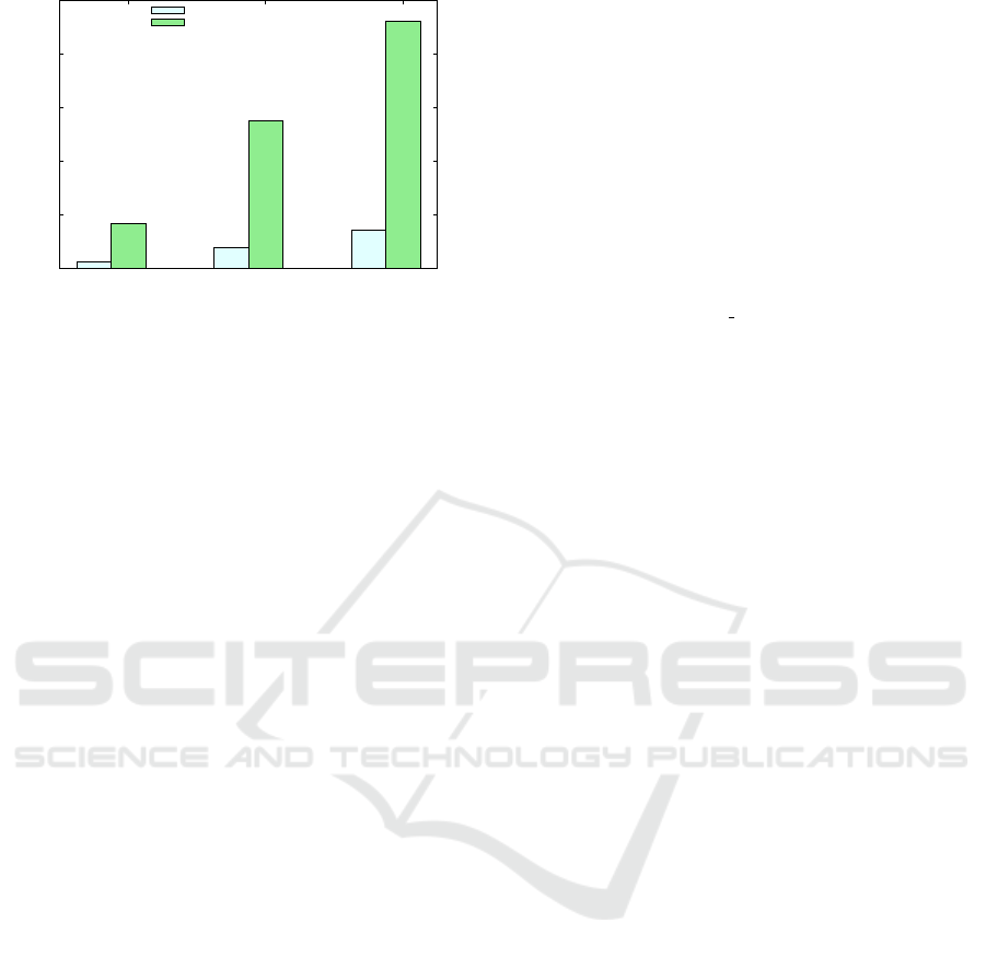
5.2.3 Random Walk vs Trafﬁc Jam

Figure 12 shows a comparison of a number of interac-

tions between vehicles using a random walk and in a

trafﬁc jam. We prepared three cases that had different

numbers of vehicles and compared the average num-

ber of interactions in the case of a random walk and

trafﬁc jam. The other conﬁguration (duration, map,

etc.) was the same as that used in the fundamental

evaluation. The number of interactions in the case of

a random walk was almost the same as the evaluation

result described in Figure 10. By contrast, the num-

ber of interactions in the case of a trafﬁc jam increased

drastically. This result indicates that almost all vehi-

cles interact with each other when they are involved

in a trafﬁc jam; hence, the trafﬁc pattern should be

created carefully so as not to induce a trafﬁc jam to

maintain the stability of the processing time.

Interaction-Based Task Group Scheduling for a Scalable and Real-Time Self-Driving Simulation

293

100

200

300

400

500

100 300 500

the number of interactions at beginning

the number of vehicles

randomwalk

traffic jam

Figure 12: Difference between the number of interactions

for a random walk and trafﬁc jam.

6 CONCLUSION

We summarize several characteristics of our approach

from the evaluation results as the following items:

• In the ideal circumstance for a self-driving simu-

lation, our approach reduced the processing time

to approximately 99 percent.

• The duration of a simulation should be less than

600 seconds in the conﬁguration of Table 2.

• We should not use our algorithm in a trafﬁc jam.

The acceptable number of vehicles in a simulation

depended on the map size. We used a map size of

2km × 2km. If the map was larger, it would be ac-

ceptable to execute more vehicles; that is, the num-

ber of interactions depended on the balance of the

number of vehicles, duration, and map size. More-

over, the acceptable number of interactions depended

on the number of CPUs in a segment. We suggested

a type of ”criterion” in our evaluation when our ap-

proach was used in a self-driving simulation to enable

it to work appropriately to maintain real-time process-

ing. We will continue to test our approach with the

other conditions

7 FUTURE WORK

An experiment on our actual self-driving simulation

cloud is obvious as a future work. There is another

major work that is to merge this priority assign ap-

proach with ”our VM deploy mechanism”. The load

balancing in our VM deploy mechanism (Kohiga and

Shinoda, 2020) is a heavy task because it utilizes VM

migration. We are thinking of an algorithm that re-

duces the number of VM migration by replacing with

this priority assign approach.

ACKNOWLEDGEMENTS

We thank Edanz (https://jp.edanz.com/ac) for editing

a draft of this manuscript.

REFERENCES

(2017). AirSim. https://microsoft.github.io/AirSim/.

(2017). Udacity’s Self-Driving Car Simulator. https://git

hub.com/udacity/self-driving-car-sim.

(2023). Incidents of Self-driving Car. https://en.wikipedia.

org/wiki/Self-driving car#Incidents.

Dahmann, J. (1997). High level architecture for simula-

tion. In Proceedings First International Workshop on

Distributed Interactive Simulation and Real Time Ap-

plications, pages 9–14.

Dosovitskiy, A., Ros, G., Codevilla, F., Lopez, A., and

Koltun, V. (2017). CARLA: An Open Urban Driving

Simulator. In Proceedings of the 1st Annual Confer-

ence on Robot Learning, pages 1–16.

Fujimoto, R. M. (2001). Parallel simulation: Parallel and

distributed simulation systems. In Proceedings of the

33nd Conference on Winter Simulation, WSC ’01,

pages 147–157, USA. IEEE Computer Society.

Kohiga, A. and Shinoda, Y. (2020). Deploy mechanism

for virtual-machine based vehicular ad hoc network

simulation. In 2020 Spring Simulation Conference

(SpringSim), pages 1–12.

Krajzewicz, D., Hertkorn, G., R

ossel, C., and Wagner, P.

(2002). Sumo (simulation of urban mobility) - an

open-source trafﬁc simulation. In 4th Middle East

Symposium on Simulation and Modelling, pages 183–

187.

Mathew, T., Sekaran, K. C., and Jose, J. (2014). Study

and analysis of various task scheduling algorithms in

the cloud computing environment. Proceedings of the

2014 International Conference on Advances in Com-

puting, Communications and Informatics, ICACCI

2014, pages 658–664.

Quigley, M., Conley, K., Gerkey, B. P., Faust, J., Foote, T.,

Leibs, J., Wheeler, R., and Ng., A. Y. (2009). ROS:

an open-source Robot Operating System. In ICRA

Workshop on Open Source Software, number Figure

1, pages 679–686.

APPENDIX

The source code of our approach.

https://github.com/akiihito/PriorityControl

SIMULTECH 2023 - 13th International Conference on Simulation and Modeling Methodologies, Technologies and Applications

294