LiDAR-GEiL: LiDAR GPU Exploitation in Lightsimulations

Manuel Philipp Vogel

, Maximilian Kunz

, Eike Gassen

and Karsten Berns

Robotics Research Lab, Dep. of Computer Science, RPTU Kaiserslautern-Landau, Kaiserslautern, Germany

Keywords:

Robotic, Simulation, Sensors, Framework, Architecture, LiDAR.

Abstract:

We propose a novel Light Detection And Ranging (LiDAR) simulation method using Unreal Engine’s Niagara

particle system. Instead of performing the ray traces sequentially on the CPU or transforming depth images

into point clouds, our method performs this particle-based approach using GPU particles that execute one

line trace each. Due to execution on the GPU, it is very fast-performing. In order to classify the results,

the new implementation is compared to existing ray-tracing and camera-based LiDAR. In addition to that

we implemented and compared common LiDAR approaches using ray-tracing as well as depth images using

cameras. A general architecture for easy exchange between simulated sensors and their communication is

given using the adapter pattern. As a benchmark, we evaluated real sensor data with a ray tracing-based

virtual sensor.

1 INTRODUCTION

Using a simulation before testing in the real world

is quite common in the ﬁeld of robotics. By doing

so, one conducts tests quickly, without the need to

travel to the testing area and set up the scenarios.

This avoids the necessity to have the robot together

with its sensors close by enabling the possibility for

parallel and distributed collaboration over long dis-

tances. Furthermore, the total control of the environ-

ment and everything within guarantees scenarios that

are not possible or too dangerous in ﬁeld tests. It is,

for example, easy to change the time of day as well as

weather conditions like rain and snow within seconds.

Regarding safety issues, testing scenarios like crashes

or incidents involving pedestrians are simulated in a

controlled environment without damaging individuals

or equipment. Another application is the generation

of training data for neural networks(Vierling et al.,

2019). Changes in lighting, viewing angles, and auto-

matically created annotations are used to create data

sets of realistic-looking images.

Since simulations are working with models of ob-

jects, there are differences from reality. They are sim-

pliﬁed illustrations compared to the represented ob-

jects (Stachowiak, 1973). Considering only the im-

https://orcid.org/0000-0000-0000-0000

https://orcid.org/0009-0006-5268-5162

https://orcid.org/0000-0002-1271-6781

https://orcid.org/0000-0002-9080-1404

portant properties, it facilitates the complexity and the

chaotic nature of the real environment. No simulation

mimics the complete state of the environment with all

its dynamic aspects and physical occurrences that can

be observed in the real world. In the case of an ideally

modeled LiDAR sensor, the simulation needs a phys-

ically correct representation of light photons. Taking

into account absorption, and reﬂection in every frame

for every sensor. Such accurate simulations are be-

yond the scope of standard hardware and require sev-

eral additional information about the environment.

In terms of computer simulation, there is a trade-

off between the complexity of the simulation and the

needed computing power and time. The optimal way

to utilize the advantages of a simulated environment

is to keep the complexity as low as needed for the

application.

The used Unreal Engine (UE)

is a game engine

developed by Epic Games

. It features real-time as

well as physical-based rendering. Providing a physics

engine, a large community, and a marketplace with

monthly free content makes it a viable simulation

software.

In this paper, UE is used for simulation of robots,

their sensors and the environments they operate in.

The implementation of the simulated sensors follows

the physical principle of the real sensors. The imple-

mented robots are digital copies of the vehicles based

https://www.unrealengine.com/en-US/

https://epicgames.com/

Vogel, M., Kunz, M., Gassen, E. and Berns, K.

LiDAR-GEiL: LiDAR GPU Exploitation in Lightsimulations.

DOI: 10.5220/0012085900003546

In Proceedings of the 13th International Conference on Simulation and Modeling Methodologies, Technologies and Applications (SIMULTECH 2023), pages 71-81

ISBN: 978-989-758-668-2; ISSN: 2184-2841

 2023 by SCITEPRESS – Science and Technology Publications, Lda. Under CC license (CC BY-NC-ND 4.0)

Table 1: Comparison of different LiDAR systems.

CPU Ray Tracing LiDAR Depth Camera LiDAR Particle LiDAR (ours)

Collision accuracy Collision Mesh Visual Depth Global Distance Fields

Performance No GPU acceleration

GPU acceleration, but overhead

from oversampling

GPU acceleration

Intensity simulation Hard (extra cameras needed) Easy Hard (extra cameras needed)

Label generation Easy Hard (needs stencil buffer) Very Hard

Simulation of rotating LiDAR Hard Very hard Easy

Noise simulation CPU bound

In parallel as post-processing of

the image

in parallel on the GPU

Modiﬁcation to Environment Avoid Foliage None

Avoid thin or very small ob-

jects/object parts

Other Problems None

Accuracy depends on bit depth

of Depth Buffer

Resolution dependent on dis-

tance to viewer.

on Computer-Aided Design (CAD) data.

2 RELATED WORK

The most common approach to simulate a LiDAR in

the UE is CARLA(Dosovitskiy et al., 2017). This plu-

gin provides the simulation of a LiDAR based on CPU

raytracing. In addition, CARLA provides other sen-

sors, such as a depth camera. Therefore, it is used for

autonomous driving simulations. To include motion

effects, LiDARsim(Manivasagam et al., 2020) intends

to build a simulation based on the real world. It sim-

ulates a LiDAR sensor including motion effects by

dividing each scan into 360 parts and simulating one

degree of the rotating LiDAR scanner in each time

step. (Hossny et al., 2020) outperformed the LiDAR

simulations by using 6 depth cameras and projecting

the images onto a sphere, where LiDAR points are

sampled. In addition to the performance improve-

ments caused by the omission of CPU ray traces, the

authors add noise textures to the depth images to ef-

ﬁciently simulate LiDAR measurement noise. (Hurl

et al., 2019) implemented a depth camera-based Li-

DAR sensor to generate a LiDAR dataset in the sim-

ulated world of the game GTA V. Another depth

camera-based approach was utilized in (Fang et al.,

2018), which also provided formulas to estimate the

intensity of the LiDAR.

2.1 Contribution

To our knowledge, we are the ﬁrst paper to exploit

GPU particles for LiDAR simulations. Additionally,

we compared the performance to different common

implementations. To quantify the virtual results, we

compared them to real sensor recordings. For better

exchangeability, we provided a general sensor archi-

tecture using the adapter pattern.

3 SENSORS

(Wolf et al., 2020) gives an overview of the already

implemented sensors in UE used by the Robotics Re-

search Lab, RPTU Kaiserslautern. New approaches

to the implementation of the sensors are described and

compared in section 3.

3.1 Structure

This subsection describes the general architecture of

our virtual sensors in the Unreal Engine. The basic

design idea is that new concepts like sensors and com-

munication principles can be integrated easily into

the existing environment without having to take care

of the basic functions. To achieve this, the adapter

design pattern was used. It provides the portability

needed for different applications. Figure 1 shows a

simpliﬁed UML diagram of the sensor design. Note

that parameters and methods have been omitted for

the sake of readability. A complete diagram can

be found on our GitHub organization

. Addition-

ally, UE-speciﬁc naming conventions were ignored

for the same reason. The detailed diagrams in ﬁg-

ure 2 show the parameters and methods as an exam-

ple. The class SensorParent is the base class for ev-

ery sensor and contains parameters and functionality

like the name of the sensor (SensorName), its repre-

sentation as a 3D model(SensorMesh) and other val-

ues like its frequency (TickIntervall). For an unam-

biguous deﬁnition of sensor parameters and the out-

put data, all sensors use structures deﬁned in the spe-

ciﬁc class (Parameters for RayTracingLiDARActor)

as input parameters and globally deﬁned output struc-

tures in the Utility class. This assures that each Li-

DAR sensor type has the same structure of its output.

That fact is used in the AdapterComponent, which

https://github.com/RRLAB-KL/Sensors

SIMULTECH 2023 - 13th International Conference on Simulation and Modeling Methodologies, Technologies and Applications

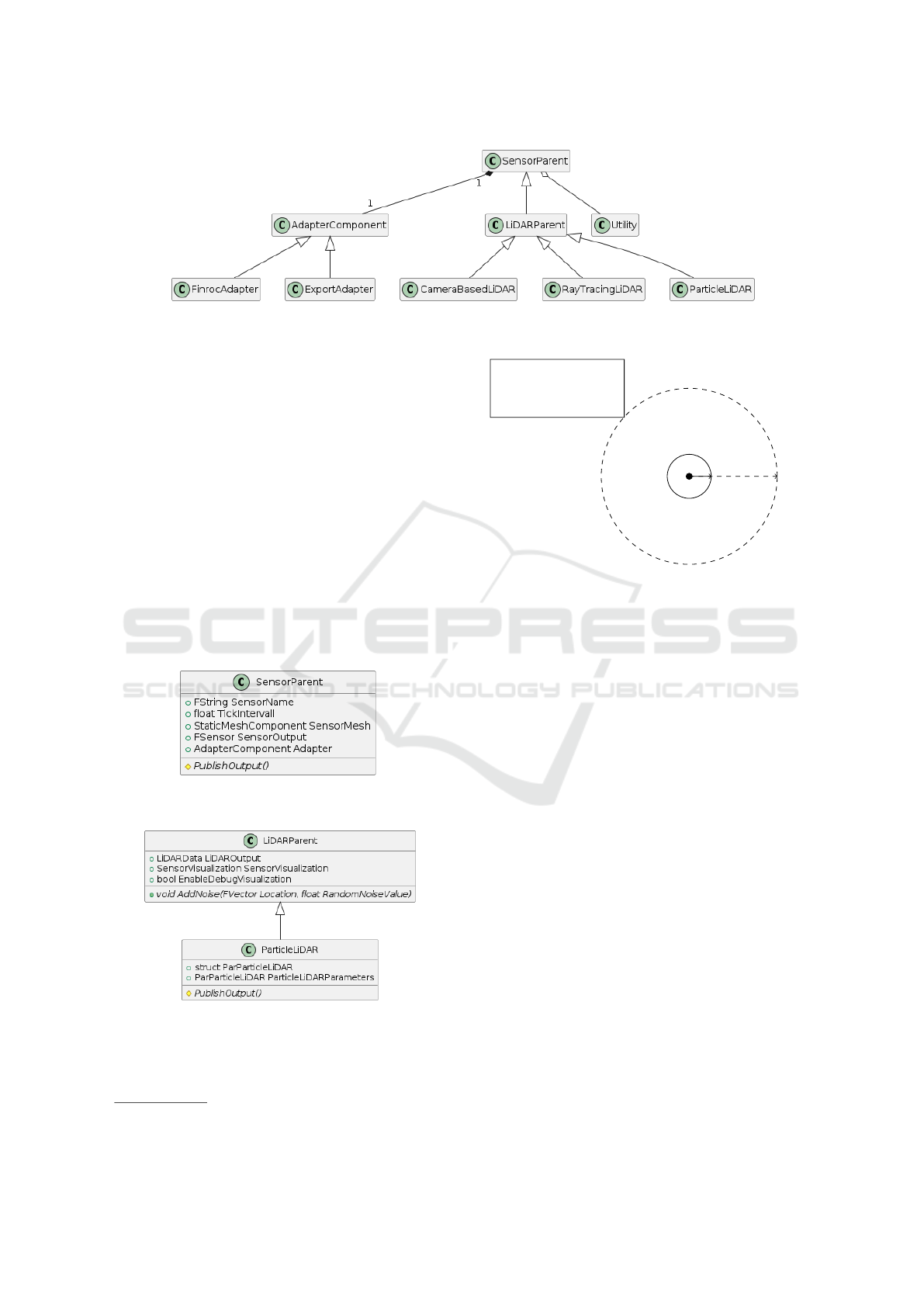
Figure 1: Simpliﬁed UML diagram of the components of the sensors as well as the adapters. A more detailed version can be

found on GitHub.

has a speciﬁc implementation in each sensor (Adapter

of the SensorParent). Independent from the speciﬁc

sensor, the method PublishLiDARData receives a Li-

DAR structure (deﬁned in Utility) as an input. The

speciﬁc behavior is implemented in the correspond-

ing adapter child class. The ExportAdapter takes the

structure and writes the points of the point cloud into

a CSV ﬁle for later processing. The FinrocAdapter

converts the unreal data to custom data types used

by our robotic framework Finroc

. The parent class

for every LiDAR-based sensor is the class LiDAR-

Parent. Here, the output structure LiDAROutput is

stored which contains the output data like an array of

3-dimensional points, the ﬁeld of view, the number of

scan lines, and additional data. The method AddNoise

uses a simpliﬁed noise model provided by the Utility

class and is overwritable.

(a) Class diagram of the SensorParent class which

is the parent class of all sensors.

(b) Class diagram of the LiDARParent and its

child, the ParticleLiDAR.

Figure 2: More detailed class diagrams of the SensorParent

and the ParticleLiDAR sensor with its direct parent.

https://www.ﬁnroc.org/

: Noise scaling

v: Random

unit vector

Figure 3: Visualization of our simple sensor model. The

input value is represented by the black dot in the center. The

vector v is the random unit vector which is multiplied by a

scaling value resulting in the vector v

which is the original

vector with additional noise.

Figure 3 shows a visualization of the sensor

model. For simplicity, only the case for 2D is consid-

ered. The raw input value is represented by the black

dot in the center. First, a random unit vector (v) is

generated which is multiplied by a noise scaling value

deﬁned by the user. The resulting vector v

represents

the original value with additional noise. The class

ParticleLiDAR shows the minimalistic setup neces-

sary for the integration in the system. They deﬁne

their speciﬁc parameters in a structure and override

the PublishOutput method based on how the point

cloud is generated. The use of the adapter pattern

in this approach has two big advantages. First, ev-

ery new LiDAR sensor is integrable into the existing

system also using every adapter as long as it stores

its values in the struct LiDAROutput and implements

the method PublishOutput. Second, if an additional

adapter is implemented, all the existing sensors are

usable. For this, the conversion of unreal data to the

new data types is deﬁned in the method PublishLi-

DARData.

LiDAR-GEiL: LiDAR GPU Exploitation in Lightsimulations

3.2 LiDAR

Different LiDAR technologies have evolved over time

(see Figure 4). The practically most used technol-

ogy is mechanically rotating LiDARs. Therefore, the

simulation of LiDAR sensors focuses on these sys-

tems. This enables the virtual testing of algorithms

in a simulated environment and the gathering of syn-

thetic data. Table 1 compares the state-of-the-art al-

gorithms with our proposed method.

Figure 4: Classiﬁcation of LiDAR systems (Wang et al.,

2020).

3.2.1 CPU Ray Tracing

The most widespread method of LiDAR simulation

is sending a speciﬁed number of traces in several di-

rections and returning to the hit location. It is deter-

mined by the intersection of one ray with an object

in the environment. Unreal Engine provides a CPU-

executed function dedicated to this purpose called

LineTraceSingleByChannel. The advantages of this

method include the high precision of the collision

point with the environment, and no communication

between GPU and CPU is needed. Additionally, the

actors at the collision point can be retrieved directly,

which allows better possibilities for recording LiDAR

datasets. Since Unreal Engine executes each line trace

sequentially on the CPU, this method results in non-

optimal performance. The second-biggest disadvan-

tage of this method is that the CPU traces collision

meshes rather than the actual visual scene. Even if

the full-scale object is used as the collision mesh, dis-

placement effects such as bump maps or tessellation

alter the scene without modifying the collision mesh.

Retrieving material properties such as roughness from

a Line Trace is not directly possible in Unreal En-

gine.Therefore, additional methods have to be used to

acquire the intensity values of the point cloud. For

example, different depth cameras are used to mea-

sure the surface properties or the amount of surface

reﬂected light. This is implemented by simulating a

light source at the position of the LiDAR. Then the

amount of reﬂected light towards it is measured (al-

though NIR light must be approximated by red light

since UE lacks NIR light simulations).

3.2.2 Depth Camera Based Techniques

A common approach to increase performance is to

eliminate the ray traces on the CPU using depth im-

ages. In depth-camera-based approaches, multiple-

depth images of the scene are rendered. The Depth

Buffer of each image is used to acquire the depth

channel of the image. Then, the RGBD image is

transformed into a 3D point cloud using the follow-

ing formulas from PseudoLidar (Wang et al., 2019):

z = Depth,

x =

(UV [0] − 0.5) · z

tan(FOV [0]) · 0.5

y =

(UV [1] − 0.5) · z

tan(FOV [1]) · 0.5

(1)

where UV∈ [0,1] is the pixel location and FOV is the

ﬁeld-of-view in the horizontal and vertical direction.

Different pixels in one row of the image correspond to

different vertical angles of the LiDAR, since the pro-

jection of vertically equal polar angles into the image

causes hyperbolic lines in the image plane (see Fig-

ure 5). Various methods have emerged to counter the

unrealistic distribution of rays that would result from

a trivial approach to map one pixel-row to a LiDAR

scan line directly. These methods include hyperbolic

approximations (Wolf et al., 2020), projections of unit

points into the images (Hurl et al., 2019), and spheri-

cal image wrapping (Hossny et al., 2020).

Figure 5: Visualization of LiDAR scan lines with 11.25°

spacing in an image with 120° FOV.

In the following section, only the projections of

unit points are considered for comparison.

Depth-Camera-based LiDAR sensors have the advan-

tage of using visual depth. This is the most accurate

representation of the scene in game engines since dis-

placement effects are also taken into account. The

SIMULTECH 2023 - 13th International Conference on Simulation and Modeling Methodologies, Technologies and Applications

disadvantages are the lower precision of the depth

at higher distances, as well as the resulting delay in

transferring images from GPU to CPU.

3.2.3 Particle LiDAR

Game engines use particles for visual effects that re-

quire a higher number of operations, but lower inter-

action between particles. The simulation of sparks

in ﬂames is one such example. The resources of the

GPU are sufﬁcient to simulate these particles entirely

and the export to the CPU takes place when the data

is needed.

Unreal Engine’s particle Engine Niagara provides

enough functionality to simulate a single laser beam

on one particle. The underlying principle of particle-

based LiDAR sensors is to ﬁrst generate particles,

each performing a line trace, calculated on GPU. Af-

terward, all collision points of the entire line traces

are exported to the CPU. This results in a high-

performance LiDAR model. It provides one of the

most efﬁcient ways of visualizing point clouds in sim-

ulation. Depending on the use case, different varia-

tions of this approach can be implemented, the basic

one is:

Algorithm 1: Basic Particle Lidar.

Input: SensorTransformation S

1 Initialization: Spawn particles

2 while sensor running do

3 Place particles in a unit sphere around S

4 for particle do

// in parallel

5 dir = particle.location expressed in S

6 LineTrace(start:S.loc, direction: dir)

7 particle.positon = LineTrace.result

8 Export positions of all particles

Instead of Algorithm 1, one can use a time interval

], split into n timesteps, and in each time step t

1/n of the traces are performed to simulate a rotating

LiDAR.

Another variant of the algorithm is to destroy par-

ticles that do not collide, and hence have the location

(0,0,0). This step is executed simultaneously for all

particles but requires the respawning of those in the

next frame.

The collision position can also be directly ex-

pressed in relation to the sensor. Thus the execution of

the transformation on the CPU is avoided. The draw-

back of this option is that the visualization of the par-

ticles does not align with the actual collision points

anymore. For example, using this variant, the particle

that collides with an object 1m in front of the sensor

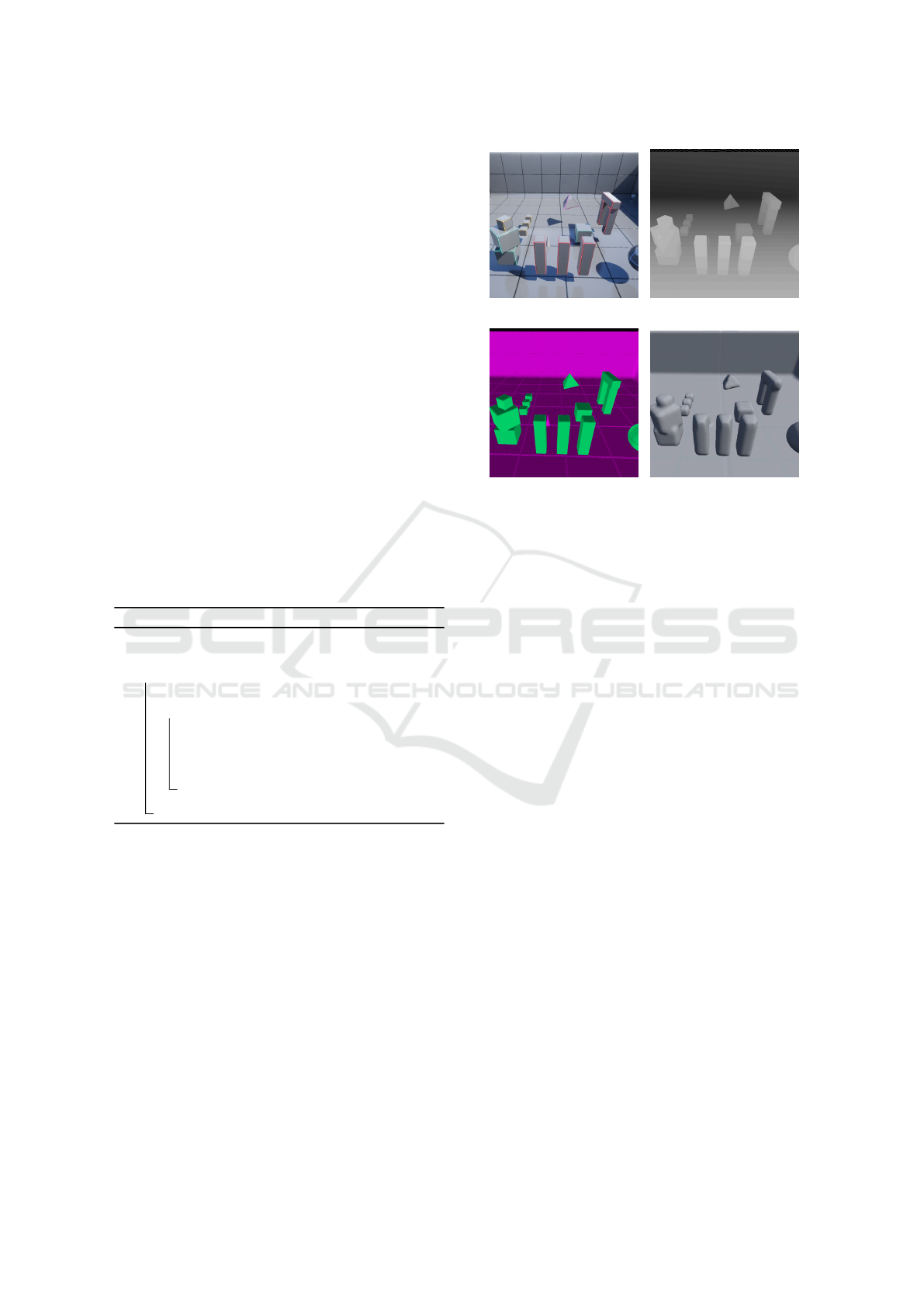
(a) Rendered Scene. (b) Scene Depth.

tance Fields.

Figure 6: Visualization of different collision methods.

would be displayed at p = (1,0,0)

in the world co-

ordinate system.

Particle Tracing. In UE, there are two types of

traces that a particle can perform. One is a spher-

ical trace for the distance ﬁelds, which is available

in UE4 and UE5. It is compatible with every op-

erating system and graphics card. Distance ﬁelds

are seen as low-resolution copies of the environment.

They are used by UE to efﬁciently simulate shad-

ows and global illumination. Although the low res-

olution of these ﬁelds greatly accelerates line traces,

the blurry geometry shapes lead to much smoother Li-

DAR point clouds compared to real ones. The alterna-

tive is the use of UE’s Hardware Ray-Tracing for col-

lision detection. It was added experimentally in the

UE5 Update but is only available on Windows with

NVIDIA RTX GPUs. This paper focuses on the for-

mer method, while the latter can be explored in the

future.

3.2.4 Comparison

Tracing Collisions. Each method of LiDAR simu-

lation uses a different method for the ray-environment

collisions, see ﬁgures 6. CPU Ray Tracing uses the

collision meshes of the object. It represents the mesh

in a detailed, yet simpliﬁed way. Depth Camera based

methods use the scene depth buffer. The particle-

based method uses the global distance ﬁelds. The

highest accuracy is performed by the depth buffer,

since it takes also displacement effects into account.

LiDAR-GEiL: LiDAR GPU Exploitation in Lightsimulations

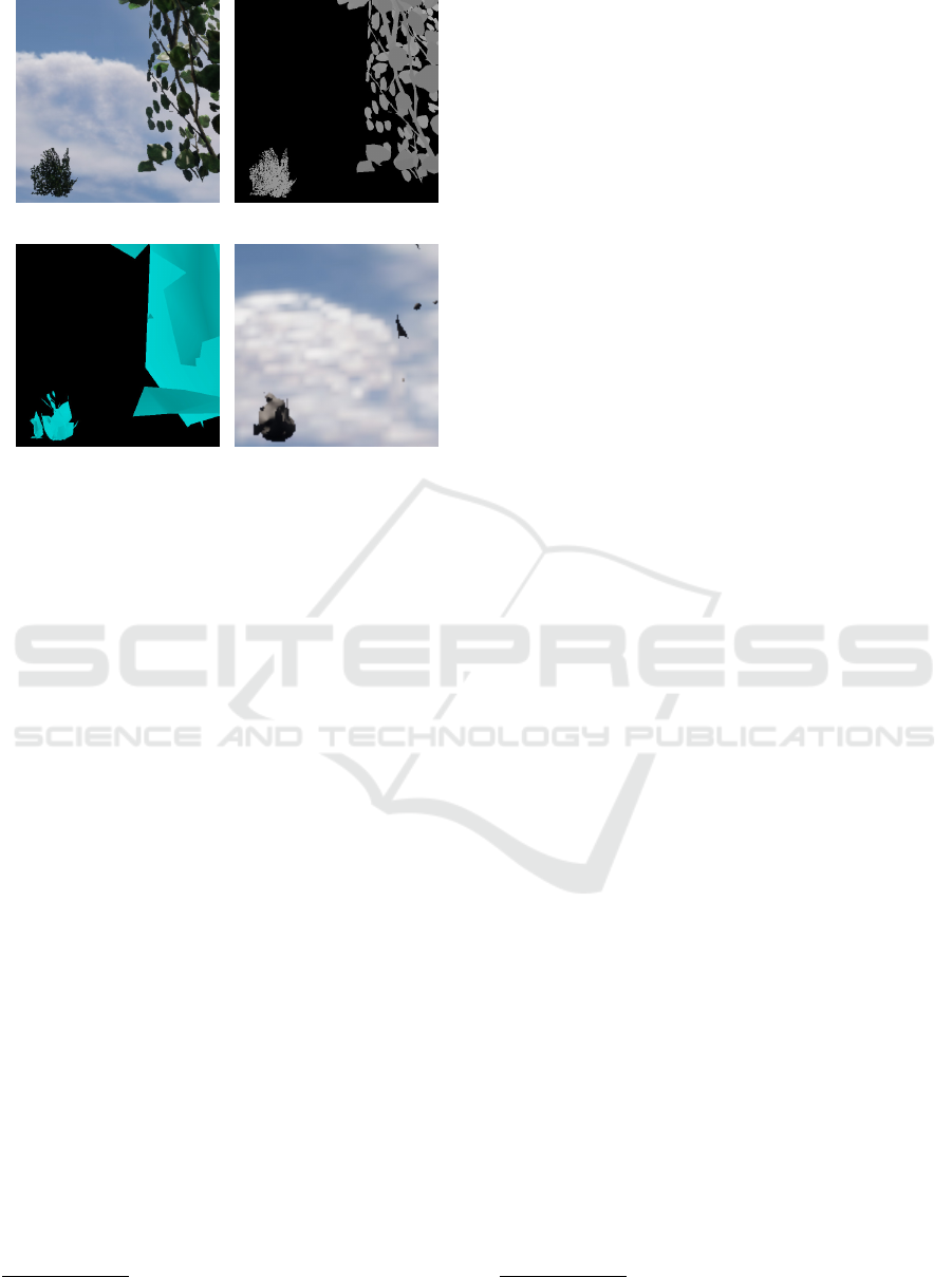
(a) Rendered Scene. (b) Scene Depth.

tance Fields.

Figure 7: Collision visualization of foliage on two different

scales. The bush consists geometrically of displaced planar

faces, which leads to problems with the mesh reconstruc-

tions from a distance ﬁeld.

This is not the case for collision meshes. In distance

ﬁelds

, the environment is split into voxels, where

each voxel stores the distance to the nearest trian-

gle. Distance ﬁelds are even less detailed than col-

lision meshes. They are meant to be a low-resolution

representation of the environment. It is used for Un-

real’s light engine Lumen and other parts that require

a resolution/performance tradeoff. The resolution of

these ﬁelds also varies based on the distance to the

viewer, and problems occur when the mesh has non-

volumetric parts, as in Figure 7.

Performance. Using the CPU for Line Tracing is

the slowest method since the traces are performed se-

quentially in Unreal Engine. However, involving the

GPU leads to communication delays because sending

information from the GPU to the CPU takes a longer

time. Depth Buffer methods have to capture and send

more information to the CPU compared to Particle Li-

DAR methods. That makes Particle LiDAR systems

the theoretically fastest method for simulation. This

enables the simulation of the motion effects of LiDAR

sensors.

Benchmarking Results (settings as in 4.1):

The time to create a point cloud is measured on an

NVIDIA A10G with a simple scene. The export of

https://docs.unrealengine.com/5.0/en-US/mesh-dista

nce-ﬁelds-in-unreal-engine/

the point cloud is not considered in the timing.

Ray Tracing: 165ms for 64 channels, 1040 ms for

512 channels

Depth Camera: 70 ms for 64 channels, 220 ms for

512 channels

GPU Particles: 42ms for 64 channels, 50 ms for 512

channels

This shows that GPU Particles are the fastest avail-

able method for generating point clouds, and that the

number of points does not affect the performance as

much as it does affect other methods. Visualizing the

points takes an additional 120 ms or >1000 ms for 64

channels or 512 channels, respectively. Only the Par-

ticle LiDAR visualizes the point cloud without perfor-

mance decreases. Hence, it is the only real-time capa-

ble method for capturing and visualizing large point

clouds

4 EXPERIMENTS

First, the simulated point clouds of the different Li-

DAR sensors are compared qualitatively. The second

part of the experiments describes the comparison be-

tween real recordings and virtual point clouds. For

this, simple objects are chosen and recreated in the

simulation. During our experiments with the virtual

sensor, it turned out that the objects we chose were

too small for the particle LiDAR and our implementa-

tion of the camera-based LiDAR. Thus, we restricted

our comparisons to the Ray Tracing sensor.

4.1 Point Cloud Difference

To measure the accuracy decrease of particle LiDARs,

we calculated the mean distance between points in a

point cloud from a Ray Tracing sensor and particle

sensors. To put that value into context, we also pro-

vide the same measurements between Ray Tracing Li-

DARs and Depth-Camera LiDARs.

4.1.1 CPU Ray Tracing

The LiDAR to represent a CPU Ray Tracing sensor

was based on CARLA’s LiDAR simulation, adapted

for native UE and without noise simulation.

4.1.2 Depth Camera LiDAR

Instead of the standard six cameras needed to render

the entire surrounding, only three with 120

◦

FOV and

The performance of GPU particle was measured with

visualizing the particles

SIMULTECH 2023 - 13th International Conference on Simulation and Modeling Methodologies, Technologies and Applications

2048x2048 resolution were used to maximize perfor-

mance.

A further improvement is the use of custom post-

processing materials. It transforms each point into 3D

local coordinates during the rendering of the image.

This also takes the rotation of two of the cameras into

account. The resulting image now has the XYZ coor-

dinates of the surface point for each pixel in the RGB

channels. Then the CPU reads the pixel values for

speciﬁc pixels and adds an offset to the coordinates.

The downside of this is that the 3D coordinates are

getting quantized.

To ﬁnd out which pixels are relevant, the horizon-

tal and vertical angles of the LiDAR scan points are

calculated. Unit vectors made of these angles are pro-

jected into the camera image. Through this, pixels

corresponding to particular LiDAR points are found.

4.1.3 Particle LiDAR

To enable meaningful benchmark, no motion effects

were simulated and algorithm 1 was used.

4.1.4 Measurement Method

Figure 8: Visualization of a point from different simulation

methods. Red: Ray tracing (used as a reference). Blue:

Depth camera approach. Orange: Particle LiDAR.

For every point in the ray tracing point cloud, we

calculated the Euclidean distance to the nearest point

in the depth camera point cloud as well as to the near-

est particle LiDAR point cloud. The distances were

then averaged. Figure 8 shows the different point

clouds. For the depth-camera based approach, the

points are forming a grid, caused by the quantization

of the XYZ values, and in the distance, each ring is

made up of straight lines due to the quantization of

the depth buffer.

Results:

Mean distance Ray Tracing LiDAR and Particle Li-

DAR:

0.936m

Mean distance Ray Tracing LiDAR and Depth Cam-

era LiDAR:

0.447m

The results from the Particle LiDAR, when assuming

the ray tracing as a reference, are worse than those

from depth camera LiDAR, but it shows, that the data

follows the same structure. However, the results de-

pend strongly on the used scene, making a standalone

statement nearly impossible.

4.2 Comparison with Real Sensors

To evaluate the different simulated sensors (see sub-

section 3.2), they are compared with a real one. A

problem is the meaningful comparison of the two

sources. It requires an accurately measured environ-

ment that is replicated in the simulation and a detailed

sensor model considering its noise. Since our noise

model is very basic, simple-shaped objects are cho-

sen as benchmarks. We measured them at different

distances from the sensor. In the real environment,

we used the Ouster OS1

laser scanner with a verti-

cal resolution of 128, a horizontal resolution of 1024

and 360

◦

ﬁeld of view. For recording, we chose three

different objects: two cardboard boxes with the di-

mensions of 237x114x179 and 322x215x295 both in

mm, as well as a bin with a diameter of 270mm and

a height of 300mm. For a qualitative comparison, we

recorded the objects, both in simulation and reality.

We alter the distances between one and six meters

with an increment of one meter. For a more robust

comparison, we recorded around ﬁve seconds of data

for every object and distance. This takes into account

noise and outliers and results in 36 recordings. The

setup is shown in ﬁgure 9.

Figure 9: Setup of our recordings. The object in the middle

laser scanner (A) in the lower left corner.

https://data.ouster.io/downloads/datasheets/datasheet-

rev7-v3p0-os1.pdf

LiDAR-GEiL: LiDAR GPU Exploitation in Lightsimulations

4.2.1 Preprocessing

Since we are only interested in the comparison of the

predeﬁned objects, the recorded point clouds have to

be preprocessed. For this, individual scans were ex-

tracted from the ﬁve-second recording. These scans

were imported into the open-source 3D modeling tool

Blender

. There, the background points were re-

moved manually. Here, we deﬁned the hull of the

recorded object and placed it at the same location as

in the recording. The overlapping points of the scan

are assumed to be the points belonging to the recorded

object. To account for the noise we increased the scale

of the object. The tolerance is around 10cm. This pro-

cess was repeated ﬁve times for every recording. 180

point clouds of the objects at varying distances and at

different times were extracted. In the simulation, we

recreated the objects and recorded them with our Ray

Tracing sensor.

4.2.2 Evaluation

For comparing the point clouds, an iterative approach

provided by the open-source Point Cloud Library

(PCL)

was used. Their Iterative Closest Point (ICP)

algorithm can be found at (ICP, ). For a comparison of

the point clouds, we used the ﬁtness score value of the

algorithm which represents the mean of squared dis-

tances between the source and reference point cloud.

Then, we analyzed the following differences:

1. Distance of same object

2. Time

3. Objects

4. Noise of the virtual sensors

4.2.3 Results

For the ﬁrst evaluation, we looked at the static noise

of the real sensor at deﬁned distances using the pre-

viously mentioned objects. In order to do this, we

compared the ﬁve-point clouds of every distance with

each other and calculated the ﬁtness score using ICP.

The resulting value is the mean squared distance for

the object at the same distance. We repeated the pro-

cess for every object at distances between 1m and 6 m.

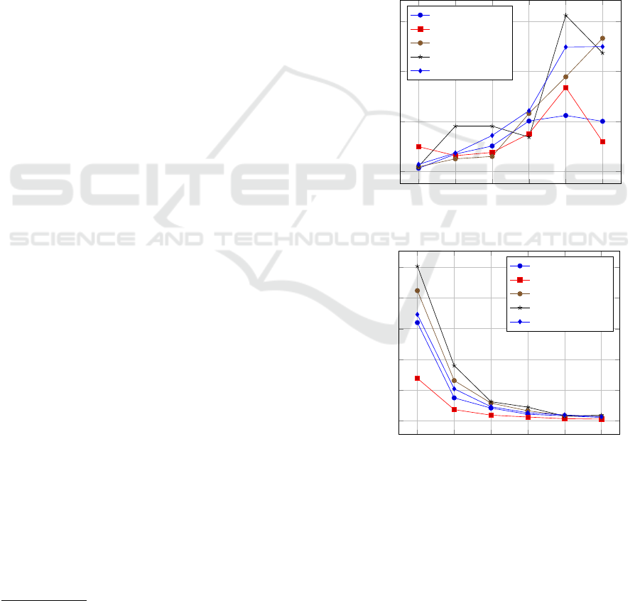
The two graphs in ﬁgure 10 show the evaluation

of these static aspects. The upper graph depicts the

mean ﬁtness score value per distance for the different

objects. Below, the corresponding number of points

of the extracted point cloud can be seen. As expected,

the number of points decreases the further the object

https://www.blender.org

https://pointclouds.org/

is from the sensor. At 5 meters, all objects have ap-

proximately the same number of points. When ex-

amining the graph in ﬁgure 10a one notices that the

mean ﬁtness score rises up to a certain point and then

decreases. One good example is the small box side

2. At 5 meters the mean ﬁtness score is at its highest

and decreases by half for 6 meters. At ﬁrst, that does

not make any sense, but when considering the lower

graph, one can see that at 6 meters the point cloud

consists of only a few points (around 6 to 10). When

looking at the recorded data, it is often the case that

the small box consists of only a single scan line. Thus,

the score value is smaller than expected because the

point clouds consist of a single line of a few points.

1 2 3 4

5 6

·10

−4

Distance

Mean ﬁtness score

small box side 1

small box side 2

large box side 1

large box side 2

bin

(a) Mean score value the objects for different distances.

1 2 3 4

5 6

200

400

600

800

1,000

Distance[m]

Number of points

small box side 1

small box side 2

große box side 1

große box side 2

bin

(b) Mean number of points of the pointclouds for differ-

ent distances.

Figure 10: Evaluation of the real recorded point clouds. The

upper graph shows the mean ﬁtness score for every object at

different distances, and the lower one the number of points

for the objects. Both distances are in meters.

For comparing the simulated point cloud with the

real recordings, we have to deﬁne a noise value based

on the simple model deﬁned in 3 using centimeter as

SIMULTECH 2023 - 13th International Conference on Simulation and Modeling Methodologies, Technologies and Applications

units. To do this, we compared the mean ﬁtness score

of the small box using the ray tracing sensor with dif-

ferent noise values at different distances. The graph

in 11 shows the results. As expected, the mean ﬁt-

ness score between consecutive scans of the same ob-

ject decreases with a higher noise value. This aspect

is intensiﬁed by the distance because the number of

points decreases the further the object is away from

the sensor which can be seen in graph (d) of ﬁgure 13.

Comparing those values with the real sensor record-

ings in ﬁgure 10 shows that the noise of it is neither

linear nor constant and we have to use different val-

ues for different distances. Having this in mind, we

increase the noise value by one centimeter for every

meter in distance for which the results of ﬁgure 11

roughly align with the real recordings in ﬁgure 10 for

the small box. In our tests, we focused on the ray-

tracing sensor since we expect that it returns the best

results in the scenario. Additionally, as explained in

subsection 3.2, small objects can not be detected by

the particle sensor and the camera based sensor. Fig-

ure 13 shows the complete evaluation for all objects at

different distances using the ray tracing LiDAR sen-

sor and the noise model explained above. The similar-

ity in the virtual and real sensor is higher than initially

expected since our linear noise model is very simple

and does not account for effects like reﬂection. Nev-

ertheless, the curves match in basic shape and also

in the absolute values besides a few outliers. These

results, however, do not show the direct comparison

of the virtual pointcloud and the real one, they only

quantify the relative accuracy of the sensors and show

that our ray tracing LiDAR with corresponding pa-

rameters has similar properties to a real sensor.

Finally, we compared the pointclouds of the vir-

tual sensor to the real data. The results can be seen

in ﬁgure 12. Here, the mean ﬁtness score between the

pointcloud of the real sensor and the ray tracing sen-

sor per object and distance can be seen. Note that the

scaling of the y axis is 10

−3

instead of 10

−4

which

was the value for the other graphs. It can be seen

that the graphs show a roughly linear behavior and

are constantly rising with some outliers. The ﬁtness

score ranges between a few millimeters at 1 meter and

around twelve centimeters at 6 meters. The high ﬁt-

ness score of the small box side 2 comes from an off-

set of the recorded object in the y axis of around 5

centimeter.

5 CONCLUSIONS

In subsection 3.1 we presented a system for adaptable

virtual sensors in Unreal Engine utilizing the adapter

1 2 3 4

·10

−4

Noise value[cm]

Mean ﬁtness score

small box side 1 1m

small box side 1 2m

small box side 1 3m

small box side 1 4m

small box side 1 5m

small box side 1 6m

Figure 11: Mean ﬁtness score value of the small box per

distance in the simulation using the ray tracing sensor using

different noise values. The noise values are in centimeter.

1 2 3 4

5 6

0.2

0.4

0.6

0.8

1.2

·10

−3

Distance[m]

Mean ﬁtness score

small box side 1

small box side 2

bin

large box side 1

large box side 2

Figure 12: Comparison between the real sensor and the vir-

tual ray tracing based LiDAR sensor for the different objects

and different distances. The noise model assumes that for

every meter one centimeter of noise is added to the current

noise value.

pattern. Its beneﬁts are easy integration of new sen-

sors as well as adaptable communication interfaces.

After that, we showed common LiDAR simulations

also introducing a new type of LiDAR simulation

method and showed that this approach is faster than

the current methods, but lacking behind in level of

detail. Although this method might be not applica-

ble for every use case, since e.g. the resolution is not

invariant to the position of the viewer, and the accu-

racy is worse than other methods, we are certain, that

the performance improvement (of ∼4x compared to

Ray Tracing) enables LiDAR sensors on much larger

scales. Lastly, we conducted experiments for com-

paring a common sensor implementation (ray-tracing

based) to a real sensor and evaluated the pointclouds

using the iterative closest points algorithm.

LiDAR-GEiL: LiDAR GPU Exploitation in Lightsimulations

5.1 Further Research

For further research, there are some aspects depend-

ing on the virtual sensor that can be improved. It is

possible to further improve the particle LiDAR ap-

proach using Hardware ray traces. Additionally, in-

stead of only considering the geometry of the scene,

we plan on developing a weighting of the sensor sig-

nals based on the material of the surface to account

for a more accurate physical model. This weighting

is predestined for the depth camera based approach

explained in subsection 4.1.2 since properties of ma-

terials can be accessed in the same way as the scene

depth in Unreal Engine. Another important aspect is

reﬂection, based on materials as well as the surface

normal. Here, the approaches vary based on the sen-

sor type, using ray-tracing it is easy to calculate re-

ﬂections. For the depth based approach, only single

reﬂections can be calculated easily since Unreal En-

gine provides a normal map of the scene similar to the

scene depth and the material properties. For all sen-

sors more work has to be invested into the noise model

to reﬂect physical properties of a LiDAR sensor.

REFERENCES

Dosovitskiy, A., Ros, G., Codevilla, F., L

opez, A. M., and

Koltun, V. (2017). Carla: An open urban driving sim-

ulator. ArXiv, abs/1711.03938.

Fang, J., Yan, F., Zhao, T., Zhang, F., Zhou, D., Yang, R.,

Ma, Y., and Wang, L. (2018). Simulating lidar point

cloud for autonomous driving using real-world scenes

and trafﬁc ﬂows.

Hossny, M., Saleh, K., Attia, M., Abobakr, A., and Iskan-

der, J. (2020). Fast synthetic lidar rendering via spher-

ical uv unwrapping of equirectangular z-buffer im-

ages. ArXiv, abs/2006.04345.

Hurl, B., Czarnecki, K., and Waslander, S. L. (2019). Pre-

cise synthetic image and lidar (presil) dataset for au-

tonomous vehicle perception. 2019 IEEE Intelligent

Vehicles Symposium (IV), pages 2522–2529.

ICP. Website of pcl icp implementation. https://pointcloud

s.org/documentation/classpcl 1 1 iterative closest p

oint.html. Accessed at 13.02.2023.

Manivasagam, S., Wang, S., Wong, K., Zeng, W.,

Sazanovich, M., Tan, S., Yang, B., Ma, W.-C., and Ur-

tasun, R. (2020). Lidarsim: Realistic lidar simulation

by leveraging the real world. 2020 IEEE/CVF Con-

ference on Computer Vision and Pattern Recognition

(CVPR), pages 11164–11173.

Stachowiak, H. (1973). Allgemeine Modelltheorie. Springer

Verlag, Wien, New York.

Vierling, A., Sutjaritvorakul, T., and Berns, K. (2019).

Dataset generation using a simulated world. In Berns,

K. and G

orges, D., editors, Advances in Service and

Industrial Robotics Proceedings of the 28th Interna-

tional Conference on Robotics in Alpe-Adria-Danube

Region (RAAD 2019), pages 505–513.

Wang, D., Watkins, C., and Xie, H. (2020). Mems mirrors

for lidar: A review. Micromachines, 11.

Wang, Y., Chao, W.-L., Garg, D., Hariharan, B., Camp-

bell, M. E., and Weinberger, K. Q. (2019). Pseudo-

lidar from visual depth estimation: Bridging the gap

in 3d object detection for autonomous driving. 2019

IEEE/CVF Conference on Computer Vision and Pat-

tern Recognition (CVPR), pages 8437–8445.

Wolf, P., Groll, T., Hemer, S., and Berns, K. (2020). Evo-

lution of robotic simulators: Using UE 4 to enable

real-world quality testing of complex autonomous

robots in unstructured environments. In Rango,

F. D.,

Oren, T., and Obaidat, M., editors, Proceed-

ings of the 10th International Conference on Simula-

tion and Modeling Methodologies, Technologies and

Applications (SIMULTECH 2020), pages 271–278.

INSTICC, SCITEPRESS – Science and Technology

Publications, Lda. ISBN: 978-989-758-444-2, DOI

10.5220/0009911502710278, Best Poster Award.

SIMULTECH 2023 - 13th International Conference on Simulation and Modeling Methodologies, Technologies and Applications

APPENDIX

Figures

1 2 3 4

5 6

·10

−4

Distance[m]

Mean Score value

small box real side 1

small box ray tracing

(a) Mean ﬁtness score of the small

box side 1.

1 2 3 4

5 6

·10

−4

Distance[m]

Mean Score value

small box real side 2

small box ray tracing

(b) Mean ﬁtness score of the small

box side 2.

1 2 3 4

5 6

·10

−4

Distance[m]

Mean Score value

large box real side 1

large box ray tracing

side 1.

1 2 3 4

5 6

100

200

300

400

500

Distance[m]

Number of points

small box real

small box ray tracing

(d) Mean number of points for the

small box side 1.

1 2 3 4

5 6

200

400

600

800

Distance[m]

Number of points

small box real side 2

small box ray tracing

(e) Mean number of points for the

small box side 2.

1 2 3 4

5 6

500

1,000

1,500

Distance[m]

Number of points

large box real side 1

large box ray tracing

(f) Mean number of points for the

small box side 1.

1 2 3 4

5 6

·10

−4

Distance[m]

Mean Score value

large box real side 2

large box ray tracing

(g) Mean ﬁtness score of the large box

side 2.

1 2 3 4

5 6

·10

−4

Distance[m]

Mean Score value

bin real

bin ray tracing

(h) Mean ﬁtness score of the bin.

1 2 3 4

5 6

500

1,000

1,500

Distance[m]

Number of points

large box real side 2

large box ray tracing

(i) Mean number of points large box

side 2.

1 2 3 4

5 6

500

1,000

1,500

Distance[m]

Number of points

bin real

bin ray tracing

(j) Mean number of points of the bin.

Figure 13: Results for the ray tracing LiDAR sensor in the Unreal Engine with different objects. The upper graphs(a-c and

g-h) show the mean ﬁtness score whereas the graphs below (d-f and i-j) shows the number of points for the object. Both, the

real data and the virtual data is shown.

LiDAR-GEiL: LiDAR GPU Exploitation in Lightsimulations