Agent Based In-Situ Visualization by Guide Field

Yan Wang

and Akira Kageyama

Graduate School of System Informatics, Kobe University, Kobe 657-8501, Japan

Keywords:

High Performance Computing, In Situ Visualization, Agent Based Modeling.

Abstract:

In situ visualization has become an important research method today in high performance computing. In our

previous study, we proposed 4D Street View (4DSV), in which multiple visualization cameras are scattered

in the simulation region for interactive analysis of visualization video ﬁles after the simulation. A challenge

in the 4DSV approach is to increase the camera density around a local area of the simulation box for detailed

visualizations. To make the cameras automatically identify such a local region or Volume of Interest (VOI), we

propose introducing the concept of a swarm of visualization cameras, which is an application of agent-based

modeling to in-situ visualization. The camera agents in the camera swarm are autonomous entities. They ﬁnd

VOIs by themselves and communicate with each other through a virtual medium called a visualization guide

ﬁeld that is distributed in the simulation space.

1 INTRODUCTION

The post hoc visualization is the standard way for

scientiﬁc visualization today, especially in high-

performance computing (HPC). A drawback of the

post hoc visualization method is that it inevitably ac-

companies massive numerical data that is to be stored

and transferred. On the other hand, the in-situ visu-

alization (Childs et al., 2020) enables directly retriev-

ing visualization images without going through mas-

sive numerical data (Bennett et al., 2018; Tikhonova

et al., 2010a; Tikhonova et al., 2010b; Ye et al., 2013;

Kawamura et al., 2016; Childs et al., 2022; Demarle

and Bauer, 2021).

A challenge in in-situ visualization is compensat-

ing for its lack of interactivity. Here, interactivity

means real-time control of visualization settings such

as viewpoint position, viewing direction, and other

parameters in terms of adopted visualization algo-

rithms, e.g., the level of the isosurface. The visualiza-

tion setting should be prescribed before a simulation

starts in the in-situ visualization.

We proposed an in-situ visualization approach that

enables interactive analysis, rather than interactive

control, of the in-situ visualization setting though vi-

sualized video ﬁles (Kageyama and Yamada, 2014).

The key idea is to apply multiple in-situ visualiza-

tions from many different viewpoints at once, then to

https://orcid.org/0000-0001-7700-0998

https://orcid.org/0000-0003-0433-668X

apply the interactive exploration of the video dataset

produced by the in-situ visualization. A similar

image-based approach to in-situ visualization is Cin-

ema (Ahrens et al., 2014; O’Leary et al., 2016). By

generalizing our video-based method, we proposed

“4D Street View (4DSV)” (Kageyama and Sakamoto,

2020; Kageyama et al., 2020), where we place thou-

sands omnidirectional cameras having a full (=4π

steradians) ﬁeld of view. The viewpoint and view-

ing direction can then be changed interactively, like

Google Street View (Anguelov et al., 2010), through

a PC application called 4D Street Viewer.

In computer simulations, visualization is com-

monly applied intensively to only a tiny portion of the

entire simulation space. We refer such a localized re-

gion as Volume of Interest (VOI) in this paper.

If the location and size of a VOI is known before

the simulation starts, we can place the visualization

viewpoints, or cameras, intensively around there. The

phenomena occurring in the VOI can be analyzed in-

teractively by the 4D Street Viewer. However, there

are possible cases where the location and motion of a

VOI is unpredictable.

A straightforward resolution for those cases is

to increase the total number of visualization cam-

eras, decreasing the distances between the cameras.

We can perform 4DSV with O(10

) omnidirectional

cameras with no problem (Kageyama and Sakamoto,

2020; Kageyama et al., 2020), but it is practically dif-

ﬁcult to increase the camera number to O(10

), or

332

Wang, Y. and Kageyama, A.

Agent Based In-Situ Visualization by Guide Field.

DOI: 10.5220/0012092800003546

In Proceedings of the 13th International Conference on Simulation and Modeling Methodologies, Technologies and Applications (SIMULTECH 2023), pages 332-339

ISBN: 978-989-758-668-2; ISSN: 2184-2841

 2023 by SCITEPRESS – Science and Technology Publications, Lda. Under CC license (CC BY-NC-ND 4.0)

more, because of computational costs.

This paper aims to propose a new method that al-

lows 4DSV with high spatial camera density with rel-

atively small number of visualization cameras, even

for unpredictable VOI behaviors.

The concept of Agent Based Visualization (ABV)

was proposed in 2017 (Grignard and Drogoul, 2017),

which combines Agent Based Model (ABM) with

information visualization in general. We proposed

an applicaiton of ABV to in-situ visualization for

HPC (Wang et al., 2022; Wang et al., 2023). In our

agent-based in situ visualization method, the agents

are visualization cameras that autonomously identify

and track VOIs by following prescribed simple rules

and applying in situ visualization.

Only the case of a single autonomous camera

tracking the motion of an unpredictable VOI was

shown in the previous work. As a natural extension,

we propose a method where multiple camera agents

follow multiple VOIs, in this paper. The challenges

here are the followings: (i) An agent should pick out

the closest VOI among multiple VOIs and get closer

to the VOI; (ii) the agent should track the VOI motion

with keeping an appropriate distance for visualiza-

tion; and (iii) agents that track the same VOI should

maintain an appropriate mutual distance each other so

as not to apply visualization of the same VOI from al-

most the same viewpoint.

In short our approach incorporates the intelligence

of a swarm into camera agents for in-situ visualiza-

tion. According to our process, camera agents can

autonomously communicate with each other and the

environment and other camera agents to determine the

location of VOI and acquire VOI-related images, al-

lowing a limited number of camera agents to acquire

more critical information about the simulated envi-

ronment.

In Section 2, we introduce the idea of agent-based

modeling (ABM) and the technical details of this

method. In Section 3, we perform test calculations

to verify the feasibility of the method proposed in this

paper. And Section 4 concludes this paper.

2 METHOD

2.1 Agent Motion

Generally, ABM consists of two parts; environment

and agents (Wilensky and Rand, 2015). According to

prescribed rules, each agent interacts with the envi-

ronment and other agents.

Our proposed method considers multiple visu-

alization viewpoints as a swarm of agents (Beni

and Wang, 1993). Rules for the camera agents

are designed to track multiple VOIs efﬁciently as a

group (Dorigo and Blum, 2005).

The environment for the camera agents is a vec-

tor ﬁeld called Visualization Guide Field (VGF) that

corresponds to the pheromones used in ABM for ant

colony (Dorigo and Blum, 2005; Deneubourg et al.,

1990; Tisue and Wilensky, 2004). Each agent moves

toward the VGF vector at its position; the VGF medi-

ates all interactions between VOI and agents as well

as among the agents.

We solve Newton’s equation of motion for each

agent, assuming that agents have unit mass. The force

acting on the agents is a function of position deter-

mined by the VGF. Additional drag force proportional

to the agent velocity is also introduced to damp high-

frequency oscillations.

Agents should have two essential traits. First,

they should move toward a nearby VOI. Second, they

should keep an appropriate distance from each other.

To achieve the dual goals, we exploit the analogy

of the electrostatic ﬁeld: The VOI has a positive elec-

tric charge +Q > 0, and the agents have a negative

charge −q < 0, where Q > q.

A negatively charged camera agent is attracted to

the positively charged VOI, and the camera agent vi-

sualizes the VOI in detail from close up. The neg-

atively charged camera agents are repelled by each

other, so they avoid the waste of being located in the

same place to visualize the same position.

The interaction between the VOI and the camera

agent is unilateral. The agent changes its position

due to the electric ﬁeld caused by the VOI’s posi-

tive charge, but the VOI is not affected by agents

even if it is closely located. In other words, the “real

space” in which the simulation is going on and the

“virtual space” in which the agents reside share the

space-time, but the interaction is one-way from the

real space to the virtual space.

We can regard the electric potential of the VGF’s

electric ﬁeld corresponds to the pheromone used

ABMs (Deneubourg et al., 1990) in general.

The location of VOIs is speciﬁed in the simulation

program in this work. The main purpose of VGF is to

attract camera agents to the speciﬁed location of VOI.

Negatively charged camera agents are automatically

attracted to the positive VOI. When there are two or

more VOIs, the VGF is given by the superposition of

ﬁelds generated by each VOI. Since VGF decays as a

function of radius in the inverse square law, an agent

is attracted naturally toward the nearest VOI.

The spherically symmetric VGF generated by a

positively charged VOI is useful when the VOI should

be visualized from a point near the VOI from any an-

Agent Based In-Situ Visualization by Guide Field

333

gle. But there are cases when some VOI should be vi-

sualized from a certain angle and the angle is known

in the simulation. For example, in a ﬂuid simulation

in which vortex-rings are spontaneously formed. The

VOI in this case can be speciﬁed in the simulation

program as the local region where the enstrophy is

spatially localized. The ring formation is detected by

the distribution of the enstrophy density in the simula-

tion. In those cases, camera agents should be attracted

to the VOI, along the axis of the ring in order to get a

better visualization of the ring formation process.

In order to guide the camera agents along a pre-

scribed direction, we introduce a dipole-type ﬁeld

as a VGF. The spherically symmetric VGF is called

monopole-type VGF.

In short, there are two types of VOI; monopole

VOI and dipole VOI. A monopole VOI is a spherically

distributed electric charge density with a net positive

charge whose origin is the center of the VOI. A dipole

VOI is a dipolar distribution of electric charge den-

sity whose moment vector is in the direction parallel

to the appropriate view-direction for the in-situ visu-

alization.

2.2 Visualization Guide Field

2.2.1 Spherical Double Layer: General Case

The dipole electric ﬁeld by a point charge has a sin-

gular behaviour near r = 0. It has inﬁnitely strong

electric ﬁeld near the point. In addition, we want the

camera agents to keep a proper distance from the VOI

center at r = 0. Because of these reasons, we realize

the monopole electric ﬁeld outside a speciﬁc radius

by assuming an inner structure of charge density dis-

tribution in the sphere.

Suppose the center of VOI, x, is at the origin, i.e.,

x = 0, and the radius of the VOI is b. We assume

a doubly layered spherical shell with the radii r = a

and r = b. We set a uniform negative charge density

−ρ

in a sphere of radius a, i.e., for radius r with 0 ≤

r ≤ a, and we set a uniform positive charge density

+ρ

in the spherical shell a < r ≤ b. We assume the

permeability ε

in the SI unit system is 1.

Applying the Gauss’ divergence theorem to the re-

lationship between the electric ﬁeld E and the charge

density ρ, i.e., ∇ ·E = ρ,

E ·r dS =

ρdV. (1)

Due to the spherical symmetry of the system, the

electric ﬁeld E caused by the spherically distributed

charge density has only the radial component E

, i.e.,

E = E

(r)

r, where

r is the radial unit vector.

The radial component is given as

(r) =











−

4πa

r (0 < r ≤ a)

4πa



r −



(a < r ≤ b)

4πa

−2a

(b ≤ r).

(2)

Here

4πa

(3)

is the total amount of charge in the sphere of r ≤ a if

constant positive charge +ρ

is uniformly distributed.

In fact, since −ρ

is distributed, the total amount of

charge in the sphere of r ≤a is −Q

. The ratio of the

two radii r = a and r = b determines the total charge in

the sphere r ≤ b and therefore the sign of the electric

ﬁeld E

(r) outside the sphere r > b. If b > b

, then

(r) > 0 for r ≥ b, where

√

2a ∼ 1.260 a (4)

Integrating eqs. (2), we get the potential φ of this

electric ﬁeld as

φ(r) =











−ρ

+ c

(0 ≤ a)

−





+ c

(a ≤ r < b)



−2a



+ c

(b ≤ r)

(5)

where c

is the integration constant.

2.2.2 Electric Field of Monopole VOI

Because there is no particular rule to determine the

value of b, we set b = b

for the monopole VOI with

√

2a ∼ 1.414 a (6)

The potential at the origin φ(0) = 0 with this b,

see eq. (2). The charge density distribution for the

monopole VOI is schematically shown in Fig. 1.

For later convenience, we explicitly write the ra-

dial electric ﬁeld of the monopole-type VOI as E

with b = b

in eqs. (2):

(r) =











−

4πa

r (0 < r ≤ a)

4πa



r −



(a < r ≤ b

)

4π

≤ r)

(7)

where

α = 2

−2 ∼0.828 (8)

The function E

(r) is monotonically decreasing

for 0 < r ≤ a, monotonically increasing for a <

r ≤ b

, and monotonically decreasing for b

< r.

) = 0.

SIMULTECH 2023 - 13th International Conference on Simulation and Modeling Methodologies, Technologies and Applications

334

Figure 1: Schematic ﬁgure for the charge density distribu-

tion of monopole-type VOI. The white dot is in the center

of the VOI, located at the origin of the two circles. The dark

blue circle with radius a has a uniform distribution of neg-

ative charges; the light blue circle between radius a and ra-

dius b

has a uniform distribution of positive charges, which

attracts the camera agent with a negative charge.

2.2.3 Electric Field of Dipole-Type VOI

The monopole VOI attracts camera agents, which are

negatively charged, and make them apply in-situ visu-

alization from all directions around the VOI’s center.

There are cases when visualizations should be ap-

plied from a speciﬁc direction and the direction is

known from the simulation program. To lead the cam-

era agents toward the desired position near the VOI’s

center to apply the in-situ visualization from the de-

sired direction, we introduce a dipole-type VOI. The

key idea is to make an electrical dipole ﬁeld outside

a sphere r = b

. The ﬁeld-lines of the dipole ﬁeld

guide the negatively charged camera agents along the

curved lines. The camera agents are naturally lead to

the positive pole of the VOI’s dipole.

As in the case of the monopole VOI, the pure

dipole causes numerical trouble due to the singular

behavior with rapidly increasing values near the ori-

gin r = 0. To avoid the problem, we introduce inner

structure inside the sphere of r = b

The potential of the dipole ﬁeld with dipole mo-

ment p is (under the assumption of ε

= 1),

4π

p ·r

(9)

which decays as a function of distance r as r

−3

for

≤ r. This is different from the r

−2

dependence of

the radial electric ﬁeld of monopole type VOI. The

difference causes an undesired behavious of a camera

agent; it can be more strongly attracted by a monopole

VOI than by a dipole VOI even the latter is closer to

the former. In order to release the difference of the r-

dependency, we use the following “quasi-dipole” po-

tential,

φ(r) =

4π

p ·r

(10)

We adopt the quasi-dipole electric ﬁeld E = −∇

φ in

r < b

Figure 2: The electric ﬁeld distribution around the dipole

VOI.

E(r) = −

4πr



p −

2(p ·r)



(11)

for b

≤ r which decays as r

−2

As for the electric ﬁeld inside the sphere of r = b

we smoothly connect the dipole ﬁeld outside r ≥ b

and a monopole-type electric ﬁeld inside r ≤ b

To put more precisely, we assume the radial elec-

tric ﬁeld by a spherical double layer of eq. (2) with

b = b

(r) =











−

4πa

r (0 < r ≤ a)

4πa



r −



(a < r ≤ b

)

(12)

Note that E

(r) = 0 for r > b

in this case of b = b

√

In the intermediate layer of b

< r ≤ b

, we as-

sume the dipole ﬁeld of eq. (11) with an attenuation

factor

H(r) =

r −b

c −b

(13)

E(r) = H(r)

E(r) (14)

in order to smoothly decay the dipole ﬁeld toward

zero at r = b

In summary, the electric ﬁeld of a (quasi-)dipole-

type VOI with pseudo-dipole moment p placed at the

origin is given by

(r) =











−

4πa

r (0 < r ≤ a)

4πa



r −



(a < r ≤ b

)

−H(r)

4πr



p −

2(p·r)



< r ≤ b

)

−

4πr



p −

2(p·r)



≤ r)

(15)

The electric ﬁeld distribution around the dipole

VOI is shown in Fig. 2, each arrow denotes the di-

rection of the electric ﬁeld.

Agent Based In-Situ Visualization by Guide Field

335

2.2.4 Multiple VOIs

In simulation in general, multiple VOIs could ap-

pear for in-situ visualizations. Suppose we place

monopole VOIs and n

dipole VOIs. We denote

VOI radius a

and the center position x

for i-th VOI

(i = 1, 2, . . . , n

). and the same for the dipole VOIs.

The relative position vector from the VOI center

to a point in the space is given by

= x −x

, (16)

with the distance

= |r

|, (17)

and unit vector

. (18)

As in the case of the real electric ﬁeld, we assume

the linearity, or superposition principle, of the electric

ﬁelds generated by multiple VOIs.

The electric ﬁeld for a camera agent at the posi-

tion x is given by the supoerposition of the monopole

ﬁelds and dipole ﬁelds as,

E(x) =

∑

i=1

)

∑

i=1

)

(19)

The computational cost of this VGF ﬁeld is negligibly

small.

3 TEST

We have performed test calculations to validate the

visualization guide ﬁeld (VGF) method described

above. The purpose of these tests are to conﬁrm

the agents motion. Visualization by these camera

agents are not considered here. Another note on

these tests are on the dimension of the computation.

In the derivations of the VGF, we assumed the 3-

dimensional space. We validate this ﬁeld on a plane

in the 3D space on which the center of VOI is located.

Assuming that all agents are on the same plane in the

initial condition, we solve the motion of the agents

only in this 2D plane.

The following test simulations are performed by

PC and the simulation programs are written in Pro-

cessing language.

3.1 Monopole VOI

Fig. 3 shows a sequence of snapshots of time devel-

opment of camera agents when we place a monopole

VOI at a ﬁxed position. Multiple agents that are

randomly distributed in the plane starts sensing the

Figure 3: The motion of camera agents when a monopole

VOI (large double circles with white and gray color) is

ﬁxed. (a) The original distribution of the camera agents.(b)

The agents are uniformly located near the monopole VOI.

monopole-type VGF and moving toward the center

of the monopole. The agents that were close to the

monopole VOI evenly distribute it at the most suit-

able distance from the monopole VOI, i.e., around the

circumference of radius b

In order to check the track-ability of agents for

moving monopole VOI, we place a moving VOI of

the monopole type. The motion of the VOI is pre-

scribed by combinations of sinusoidal functions of

time in these tests.

Fig. 4 shows a time sequence from a period, the

monopole VOI oscillates horizontally in this case.

The camera agents that were initially distributed

about the whole plane are attracted to the VOI and

they follow a little behind the VOI as a group.

We have also performed tests in two dimensional

monopole VOI motion, conﬁrming that the agents can

track the VOI motion as long as the VOI speed is not

too high.

We also performed tests when the monopole VOI

makes random movements. the camera agents can

successfully ﬁnd and track the monopole VOI as

shown in Fig. 5.

3.2 Dipole VOI

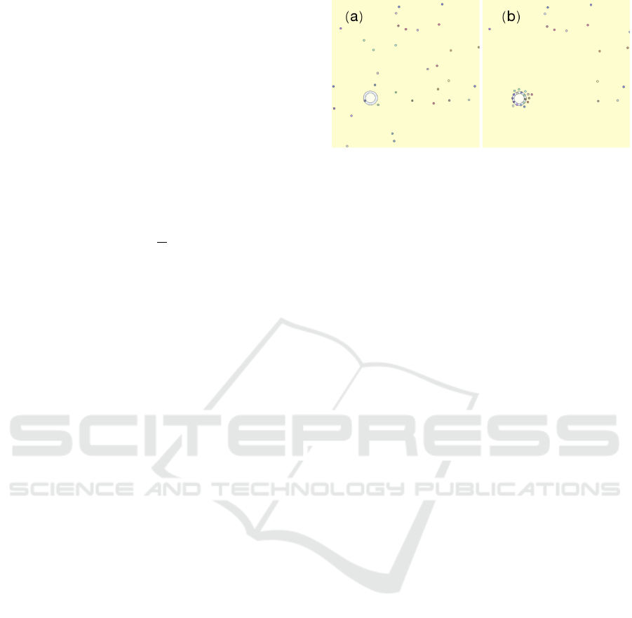
Fig. 6 shows a snapshot when a dipole-type VOI is

placed on the plane. The dipole moment is indi-

cated by arrow in the VOI circle. The camera agents

that were randomly distributed in the initial condition

senses the dipole ﬁeld and move along the ﬁeld-line.

They eventually accumulate around the “pole” of the

dipole. This is the desired behaviour of the agents

to realize the in-situ visualization of the VOI from a

speciﬁc angle.

As shown in Fig. 7, when the dipole VOI does

random motion, the camera agent can still detect and

track the dipole VOI in time and can maintain a spe-

ciﬁc view of the dipole VOI.

SIMULTECH 2023 - 13th International Conference on Simulation and Modeling Methodologies, Technologies and Applications

336

Figure 4: Camera agents when a monopole VOI is making a

one-dimensional harmonic oscillation. (a) The original dis-

tribution of the monopole VOI and camera agents; (b) to (h)

The camera agents gradually converging to the monopole

VOI and following a little behind it as a group. (i) and (j)

The camera agents successfully track the orbit of the VOI,

but the lag becomes larger for a faster-moving VOI.

3.3 Multiple VOIs

The next experiment is to take into account how the

camera agent will move when multiple monopole

VOIs are present at the same time. As shown in Fig. 8,

when three monopole VOIs appear at the same time,

the camera agent will autonomously ﬁnd the closest

monopole VOI to it and follow it. As in the case of

the single VOI case, the camera agents can follow the

multiple VOIs even if they are moving. And, as the

Figure 5: Camera agent when a monopole VOI makes ran-

dom motion. (a) The original distributions; (b) Gradual ag-

gregation of the camera agents toward the monopole VOI;

monopole VOI.

Figure 6: Camera agent when a dipole VOI is ﬁxed. (a)

The original distributions. (b) The agents are attracted to

the dipole VOI from a speciﬁc direction.

position of the monopole VOI changes, the camera

agent can always choose to change the target to fol-

low, tracking a closer VOI.

The ﬁnal test shown is Fig. 9 in which a monopole

VOI and a dipole VOI are present at the same time,

the camera agents still ﬁnd the closest VOI and tracks

them autonomously.

Agent Based In-Situ Visualization by Guide Field

337

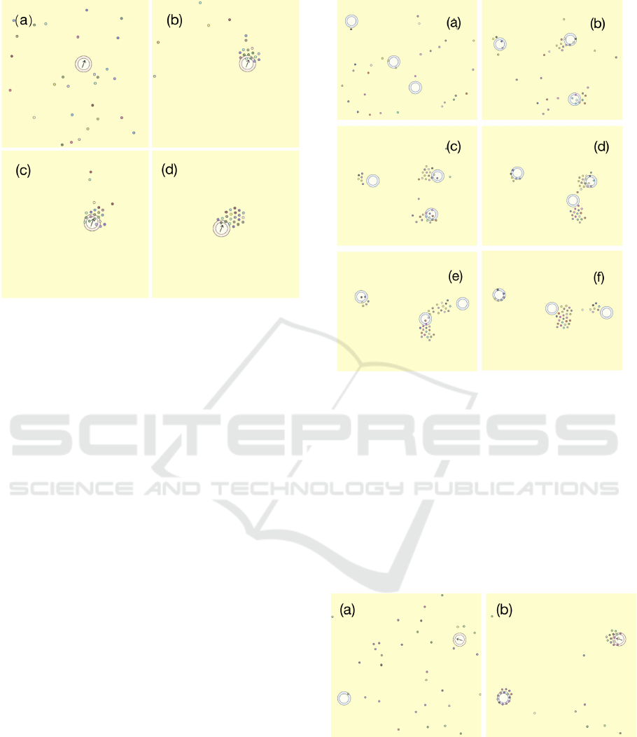
Figure 7: The camera agent when a dipole VOI does ran-

dom motion. (a) The original distributions. (b) The camera

agents converge near the dipole VOI from a speciﬁed di-

rection. (c) The camera agents are aggregated in a suitable

position, or the “pole”, to observe the VOI from a proper

viewing direction. (d) The agents continue to follow the

VOI in motion.

4 CONCLUSIONS

We propose an agent based visualization approach

to in-situ visualization for computer simulations. In

this method, camera agents in a “camera swarm”

communicate with each other and with the environ-

ment through a vector ﬁeld, Visualization Guide Field

(VGF).

The volume of interest (VOI) that should be ap-

plied intensive visualization is a source of VGF in our

method. Inspired by the static electric ﬁeld, a VOI

that should be a focus of intensive visualization is a

positively changed object and a visualization camera

is a negatively charged object. The camera is a mov-

able entity and called camera agent.

VOI can be either monopole-type or dipole-type.

The monopole-type VOI corresponds to a local region

where in-situ visualization should be applied in close-

up, but from any direciton. The dipole-type VOI cor-

responds to a local region that should be visualized

from a speciﬁc angle.

According to the repulsive force between agents,

they can keep a proper distance even if they are at-

tracted to the same VOI.

Our approach will improve the visualization efﬁ-

ciency by allowing camera agents to autonomously

ﬁnd and track VOI, reducing the number of cameras

Figure 8: Motion of the camera agent when the monopole

VOIs do random motion. (a) shows the original distribu-

tion of monopole VOI and camera agents; (b) shows that

camera agents gradually converge to the nearest monopole

VOI; (c) shows that camera agents will follow the monopole

VOI motion after converging near their respective near-

est monopole VOI. The colors of the camera agents are

set randomly to facilitate observation, and different cam-

era agents will select the closer monopole VOI for observa-

tion. (d),(e) show that the camera agents may also reselect

the monopole VOI to be observed based on the distance af-

ter the monopole VOI motion produces an intersection. (f)

shows that the camera agents will continue to steadily fol-

low the selected monopole VOI after reselection.

Figure 9: Motion of the camera agent when a monopole

VOI and a dipole VOI are present at the same time. (a)

shows the original distribution of VOIs and camera agents;

(b) shows when camera agents are distributed around each

VOI according to the demand of different VOIs.

set up in the simulated environment and allowing us

to obtain data focused on the region of interest rather

than the background region.

SIMULTECH 2023 - 13th International Conference on Simulation and Modeling Methodologies, Technologies and Applications

338

ACKNOWLEDGEMENTS

This work was supported by JSPS KAKENHI (Grant

Numbers 22H03603, 22K18703).

REFERENCES

Ahrens, J., Jourdain, S., O’Leary, P., Patchett, J., Rogers,

D. H., and Petersen, M. (2014). An Image-Based ap-

proach to extreme scale in situ visualization and anal-

ysis.

Anguelov, D., Dulong, C., Filip, D., Frueh, C., Lafon,

S., Lyon, R., Ogale, A., Vincent, L., and Weaver, J.

(2010). Google street view: Capturing the world at

street level. Computer, 43(6):32–38.

Beni, G. and Wang, J. (1993). Swarm intelligence in cel-

lular robotic systems. In Dario, P. and others, editors,

Robots and Biological Systems: Towards a New Bion-

ics?, pages 703–712. Springer-Verlag Berlin Heidel-

berg.

Bennett, J. C., Childs, H., Garth, C., and Hentschel, B.

(2018). In Situ Visualization for Computational Sci-

ence. In Situ Vis. Comput. Sci. Dagstuhl Semin. 18271,

volume 8, pages 1–43.

Childs, H., Ahern, S. D., Ahrens, J., Bauer, A. C., Bennett,

J., Bethel, E. W., Bremer, P.-T., Brugger, E., Cottam,

J., Dorier, M., Dutta, S., Favre, J. M., Fogal, T., Frey,

S., Garth, C., Geveci, B., Godoy, W. F., Hansen, C. D.,

Harrison, C., Hentschel, B., Insley, J., Johnson, C. R.,

Klasky, S., Knoll, A., Kress, J., Larsen, M., Lofstead,

J., Ma, K.-L., Malakar, P., Meredith, J., Moreland, K.,

Navr

atil, P., O’Leary, P., Parashar, M., Pascucci, V.,

Patchett, J., Peterka, T., Petruzza, S., Podhorszki, N.,

Pugmire, D., Rasquin, M., Rizzi, S., Rogers, D. H.,

Sane, S., Sauer, F., Sisneros, R., Shen, H.-W., Usher,

W., Vickery, R., Vishwanath, V., Wald, I., Wang, R.,

Weber, G. H., Whitlock, B., Wolf, M., Yu, H., and

Ziegeler, S. B. (2020). A terminology for in situ visu-

alization and analysis systems. Int. J. High Perform.

Comput. Appl., 34(6):676–691.

Childs, H., Bennett, J. C., and Garth, C., editors (2022).

In Situ Visualization for Computational Science.

Springer International Publishing.

Demarle, D. E. and Bauer, A. (2021). In Situ Visualization

with Temporal Caching. Comput. Sci. Eng., 23:25–33.

Deneubourg, J.-L., Aron, S., Goss, S., and Pasteels, J. M.

(1990). The self-organizing exploratory pattern of the

argentine ant. J. Insect Behav., 3(2):159–168.

Dorigo, M. and Blum, C. (2005). Ant colony optimization

theory: A survey. Theor. Comput. Sci., 344(2-3):243–

278.

Grignard, A. and Drogoul, A. (2017). Agent-Based vi-

sualization: A Real-Time visualization tool applied

both to data and simulation outputs. In The AAAI-17

Workshop on Human-Machine Collaborative Learn-

ing, pages 670–675.

Kageyama, A. and Sakamoto, N. (2020). 4D street view: a

video-based visualization method. PeerJ Comput Sci,

6:e305.

Kageyama, A., Sakamoto, N., Miura, H., and Ohno, N.

(2020). Interactive exploration of the In-Situ vi-

sualization of a magnetohydrodynamic simulation.

Plasma and Fusion Research, 15:1401065–1401065.

Kageyama, A. and Yamada, T. (2014). An approach to ex-

ascale visualization: Interactive viewing of in-situ vi-

sualization. Comput. Phys. Commun., 185(1):79–85.

Kawamura, T., Noda, T., and Idomura, Y. (2016). In-situ

visual exploration of multivariate volume data based

on particle based volume rendering. In 2nd Work. Situ

Infrastructures Enabling Extrem. Anal. Vis., pages 18–

22.

O’Leary, P., Ahrens, J., Jourdain, S., Wittenburg, S.,

Rogers, D. H., and Petersen, M. (2016). Cin-

ema image-based in situ analysis and visualization of

MPAS-ocean simulations. Parallel Comput., 55:43–

48.

Tikhonova, A., Correa, C. D., and Kwan-Liu, M. (2010a).

Explorable images for visualizing volume data. Proc.

IEEE Paciﬁc Vis. Symp. 2010, PaciﬁcVis 2010, pages

177–184.

Tikhonova, A., Correa, C. D., and Ma, K. L. (2010b). Vi-

sualization by proxy: A novel framework for deferred

interaction with volume data. IEEE Trans. Vis. Com-

put. Graph., 16(6):1551–1559.

Tisue, S. and Wilensky, U. (2004). NetLogo: Design

and implementation of a multi-agent modeling envi-

ronment. In Proceedings of the Agent 2004 Confer-

ence on Social Dynamics: Interaction, Reﬂexivity and

Emergence.

Wang, Y., Ohno, N., and Kageyama, A. (2023). In situ vi-

sualization inspired by ant colony formation. Plasma

and Fusion Research, 18:2401045.

Wang, Y., Sakai, R., and Kageyama, A. (2022). Toward

agent-based in situ visualization. In By, C. and Choi,

C., editors, Methods and Applications for Modeling

and Simulation of Complex Systems. CCIS, 1636.

Wilensky, U. and Rand, W. (2015). An Introduction to

Agent-Based Modeling: Modeling Natural, Social,

and Engineered Complex Systems with NetLogo. MIT

Press.

Ye, Y., Miller, R., and Ma, K.-L. (2013). In situ pathtube

visualization with explorable images. In 13th Euro-

graphics Symp. Parallel Graph. Vis., pages 9–16. Eu-

rographics Association.

Agent Based In-Situ Visualization by Guide Field

339