A Concept for Optimizing Motor Control Parameters Using Bayesian

Optimization

Henning Cui

1 a

, Markus G

orlich-Bucher

1 b

, Lukas Rosenbauer

, J

org H

ahner

1 c

and Daniel Gerber

Organic Computing Group, University of Augsburg, Am Technologiezentrum 8, 86159 Augsburg, Germany

BSH Hausger

ate GmbH, Im Gewerbepark B35, 93059 Regensburg, Germany

Keywords:

Bayesian Optimization, DC-Motor, Motor Control, Multiple-Objective, NSGA-II.

Abstract:

Electrical motors need speciﬁc parametrizations to run in highly specialized use cases. However, ﬁnding such

parametrizations may need a lot of time and expert knowledge. Furthermore, the task gets more complex as

multiple optimization goals interplay. Thus, we propose a novel approach using Bayesian Optimization to ﬁnd

optimal conﬁguration parameters for an electric motor. In addition, a multi-objective problem is present as two

different and competing objectives must be optimized. At ﬁrst, the motor must reach a desired revolution per

minute as fast as possible. Afterwards, it must be able to continue running without ﬂuctuating currents. For

this task, we utilize Bayesian Optimization to optimize parameters. In addition, the evolutionary algorithm

NSGA-II is used for the multi-objective setting, as NSGA-II is able to ﬁnd an optimal pareto front. Our

approach is evaluated using three different motors mounted to a test bench. Depending on the motor, we are

able to ﬁnd good parameters in about 60-100%.

1 INTRODUCTION

Many new trends, such as e-mobility, highly rely on

advanced electrical machines. This is also the case for

many everyday devices such as washing machines.

These modern electrical machines rely on com-

plex motor control algorithms and software. Further-

more, motors are usually ﬁne-tuned by an electrical

engineer with years of experience in motor develop-

ment. Such optimization can be important, as choos-

ing wrong parameters may lead to time loss, a failure

to run the motor correctly, or even damage it. This,

however, is a complex task as many different param-

eters interplay in a wide range. In addition, ﬁnding

good parameters require highly speciﬁc expert knowl-

edge, which can be very expensive. Furthermore,

such expert knowledge might not even be available

considering older machines. It is also possible that

such expert knowledge does not lead to the best per-

formances. Due to different inﬂuences like the en-

vironment, load or wear, an optimal conﬁguration of

a system might change or must even be reconﬁgured

https://orcid.org/0000-0001-5483-5079

https://orcid.org/0000-0002-2036-0308

https://orcid.org/0000-0003-0107-264X

during runtime.

For that reason, we present a novel approach for

optimizing the parametrization of different electrical

motors given two competing goals. The ﬁrst goal is

for the motor to achieve a predeﬁned revolutions per

minute (RPM) as fast as possible. Afterwards, the

second objective is for the motor to maintain the RPM

with as little ﬂuctuation in its current ripple as possi-

ble. A very fast start may lead to a motor running

unstable after reaching its RPM, as its parametriza-

tion is only optimized for a fast startup. Hence, the

parametrization for maintaining the RPM may not be

optimal which could lead to a higher energy consump-

tion.

For our methodology, we utilize Bayesian Opti-

mization (Mockus, 2012) to optimize the parametriza-

tion. As for multiple, competing objectives, the evolu-

tionary algorithm NSGA-II (Deb et al., 2002) is used.

Following, in Section 2, we give a brief overview

of existing related work. We explain our used mo-

tor test bed in Section 3 before outlining the overall

problem in Section 4. Afterwards, we provide a brief

introduction to Bayesian Optimization in Section 5.

Finally, we evaluate our approach in Section 6 before

concluding with an outlook on possible future work

in Section 7.

Cui, H., Görlich-Bucher, M., Rosenbauer, L., Hähner, J. and Gerber, D.

A Concept for Optimizing Motor Control Parameters Using Bayesian Optimization.

DOI: 10.5220/0012093700003543

In Proceedings of the 20th International Conference on Informatics in Control, Automation and Robotics (ICINCO 2023) - Volume 1, pages 107-114

ISBN: 978-989-758-670-5; ISSN: 2184-2809

107

2 RELATED WORK

Various relevant previous work on using Bayesian

Optimization for different kinds of machinery ex-

ists. Notable examples focus on optimizing the be-

haviour of robots, e.g. (Akrour et al., 2017). These

approaches, however, vary from our concept such that

we focus solely on conﬁguring and optimizing param-

eters that need to be set in order to able to use the mo-

tor, instead of optimizing the behaviour of a complex

machinery as whole.

The authors of (Khosravi et al., 2021) tune a motor

with the Bayesian optimizer as well. However, they

focus on optimizing industrialized brushless motors.

We on the other hand utilize DC-motors, a completely

different kinds of motor, and consider the whole con-

trol scheme as a black box which they do not.

Another work from Neumann-Brosig et

al. (Neumann-Brosig et al., 2020) uses Bayesian

Optimization in an industrial setting. They optimize

parameters for a throttle valve control. While the

throttle valve control contains a DC motor, they do

not directly optimize motor parameters. Instead,

their motor is only indirectly inﬂuenced by their

parametrization by factors like the voltage input.

onig et al. (K

onig et al., 2021) utilizes Bayesian

Optimization to ﬁnd optimal motor parameters, too.

However, we differ from their work as they based

their work on an AC motor while we utilize a DC mo-

tor. Furthermore, they do not aim to optimize speed

and voltage ﬂuctuation but to maximize tracking ac-

curacy.

Other noteworthy works focus on automatically

improving motors with various other methods. Na-

ture inspired swarm algorithms like the artiﬁcial bee

colony algorithm or the ﬂower pollination algorithm

can be used to tune parameters, as was done in (Tar-

czewski and Grzesiak, 2018). Alternatively, the par-

ticle swarm optimization algorithm can be used, too,

as was done by (Sharma et al., 2022) or (Naidu Kom-

mula and Reddy Kota, 2022). Other metaheuristics

can be used too, like the grey wolf optimizer (Kamin-

ski, 2020). It is also possible to use specialized opti-

mization algorithms, like an adaptive safe experimen-

tation dynamics method (Ghazali et al., 2022).

3 TEST BED

In the following, we introduce our test environment

now to better understand the optimization problems

we are going to introduce in the next Section 4. Our

test bed contains different hardware objects, each per-

forming one or multiple functionalities. An abstracted

PC (1)

Dynamometer \

Controller (3)

Inverter \

Motor Control (4)

Oscilloscope (2) Power Supply (5)

DC-Motor (6)

Figure 1: An abstracted overview of the test bed.

view of our setup can be seen in Figure 1. The com-

puter is a standard desktop PC on which our software

and optimizer runs. It is connected to an oscilloscope,

an inverter, a power supply for the inverter and motor

as well as a dynamometer and its controller.

The oscilloscope measures the current ripple for a

sampling rate f

. This is important as we need this

information for the second objective deﬁned in Sec-

tion 4.

The inverter is build with a motor control unit and

controls the DC-motor driven by the direct current

(DC) as well as the power supplied to it. Thus, the

inverter handles the angular acceleration as well. It

receives a set of parameters from the PC to indirectly

control the speed up of the motor by changing the fre-

quency of power supplied. Another utility is setting

the desired RPM as well as starting and stopping the

motor.

The motor control tool is powered by the power

supply.

Another hardware object is the dynamome-

ter (Magtrol Inc., 2022b) and its controller (Magtrol

Inc., 2022a). They are used to accurately read out the

RPM.

At last, we tested our setup on three different mo-

tors. We use electric motors which are driven by an

direct current build for household appliances. Mo-

tor 2 and 3 have a smaller or larger axial impeller to

simulate a load. Thereby we have a more realistic,

real world motor setting. The ﬁrst motor on the other

hand does not utilize an axial impeller. The motors

itself are connected to the oscilloscope, inverter and

dynanometer to read out useful information for the

optimization process.

4 PROBLEM DESCRIPTION

In our work, we consider two different problem

descriptions. Both problems have in common that we

want to optimize 11 parameters in a speciﬁc interval.

They control the behaviour of motors such as the

angular acceleration which deﬁnes how fast the motor

speeds up, its current ripple, etc.. As we assume no

further expert knowledge about these parameters—

with the system as a whole being seen as a black-

ICINCO 2023 - 20th International Conference on Informatics in Control, Automation and Robotics

108

box—we do not discuss the parameters in more

detail.

4.0.1 Optimization Problem 1

Our ﬁrst optimization problem is single objective

where we only consider the angular acceleration of

the motor. The goal is to reach a ﬁxed rounds

per minute (RPM) as fast as possible. Let p =

{

, . . . , p

}

and t

(p) be the time it takes for the

motor to reach the desired RPM given a set of param-

eters with p ∈ X and X ⊂ R

. Then our ﬁtness value

is the deﬁned time:

(p) = t

(p) (1)

This leads us to the following optimization problem:

min

p∈X

(p) (2)

4.0.2 Optimization Problem 2

The next use case we consider is a biobjective opti-

mization problem. At ﬁrst, the motor should acceler-

ate as fast as possible. Furthermore, after it reaches its

desired angular speed, the current ripple (CR) should

be as consistent as possible. As the motor runs, it re-

quires continuous power due to frictions, resistances,

loads, etc. to keep its RPM. With an inconsistent CR,

multiple problems might occur such as the motor fail-

ing to keep spinning or a decrease of efﬁciency due to

the excessive energy being dissipated in the form of

heat. Thus, the lifespan of a motor is shortened, too

Thus, we extend our ﬁtness function from Equa-

tion 1. Let I

(p) be the current ripple of timestep t

given parameters p and I =

{

, . . . , I

}

. Furthermore,

Var(X) is the variance of a random variable X. Then,

our second ﬁtness function f

is deﬁned as follows:

(p) = Var (I (p)) (3)

Thus, we extend our optimization problem from

Equation 2:

min

p∈X

( f

(p), f

(p)) (4)

5 BAYESIAN OPTIMIZATION

Bayesian Optimization (BO) is a global optimization

method (Mockus, 2012). As is seen in Section 3, we

have a hardware in the loop system consisting of a

motor, its controlling mechanism and a RPM mea-

surement system. Furthermore, the system is seen

as a black-box. BO is a good choice for our setting,

as Jones et al. (Jones et al., 1998) describes BO as a

good black-box optimizer, as no prior insight about

the ﬁtness landscape is needed. Additionally, BO is

even able to ﬁnd a global optimum in the presence of

stochastic noise (Mockus, 2012)—which occurs with

our use case. At last, there is still the issue that one

evaluation could take several minutes. While BO is

not able to ﬁx this problem, the optimization algo-

rithm is able to handle the limitation of a costly eval-

uation function well (Brochu et al., 2009).

5.1 Introduction to Bayesian

Optimization

In Bayesian Optimization, we try ﬁnd a global max-

imizer (or minimizer) of an unknown objective func-

tion f . This optimum is found by utilizing every value

of previous evaluation points. For this task, BO needs

a prior which describes the objective function f for

now. In this context of BO, the prior is a function

which describes the beliefs about the behaviour of

the unknown function. Furthermore, an acquisition

function is needed which decides the next sampling

point (Jones, 2001; Snoek et al., 2012).

5.1.1 Gaussian Process Prior

To describe our searched-for function f , BO creates a

Gaussian process (GP) from which a distribution over

functions is derived. Such a distribution over func-

tions means that we do not calculate a single scalar

output for a given input. Instead, we get the mean and

variance of a normal distribution describing possible

values for a given input (Frazier, 2018). By utilizing

a distribution of functions, GP is able to express un-

certainties. As a result of this trade off, BO is able

to optimize the objective function with fewer evalua-

tions needed (Shahriari et al., 2016).

To utilize a GP, a kernel function is needed as

well. The kernel describes the correlation between

two points in the input space. In our implementation,

we utilize the Mat

ern covariance function k

(Ras-

mussen, 2003) as a kernel function as it shows prefer-

able properties, like being able to model physical pro-

cesses well (Rasmussen, 2003; Shahriari et al., 2016).

5.1.2 Acquisition Function

The acquisition function α (·) is another important

part of BO as it determines which data point to ob-

serve next. The main idea is to choose a point based

on a high uncertainty of the GP function or where the

objective function has a potentially high value.

However, choosing the right acquisition function

is no trivial task and requires a lot of evaluation.

Thus, we adopt scikit-learns (Buitinck et al., 2013)

A Concept for Optimizing Motor Control Parameters Using Bayesian Optimization

109

strategy of utilizing three different acquisition func-

tions: Probability of Improvement (Kushner, 1964),

Expected Improvement (Mockus, 1975) and Upper

Conﬁdence Bound (Cox and John, 1992). They op-

timise each acquisition function independently and

at each step all three functions propose an candidate

point. The next observation point is then chosen prob-

abilistically by choosing the point with the highest

gain.

To better visualize the concept of BO, we exem-

pliﬁed this concept in Figure 2. It shows an example

of BO on an 1D objective function, calculated over

4 iterations. Each sub-ﬁgure is partitioned into two.

The top image shows the true objective function f

(red line), the Gaussian process model (green area)

and its estimation of f (green dashed line). Further-

more, it shows new (magenta points) and old obser-

vation points (dark green) if existing. The bottom ﬁg-

ure shows the correlating acquisition function f

(blue

line) and the next point to sample (blue ’x’). Figure 2a

shows step 0 after its initialization. We sampled 5 ran-

dom points to create our GP as well as α (·). Now, we

choose our next sampling point. The next Figure 2b

shows the observed sampling point as well as an up-

dated GP model and acquisition function. We then

repeat these steps multiple times to ﬁnd the global op-

timum.

For a more indepth view of BO, we refer to the

works of Brochu et al. (Brochu et al., 2009), Shahriari

et al. (Shahriari et al., 2016) and Mockus (Mockus,

2012).

5.2 Multi-Objective Bayesian

Optimization

As is described in section 3, another goal is to opti-

mize multiple objectives. New challenges arise with

a multi-objective as we have to ﬁnd the Pareto Set

which is a set of solutions where all objectives are

optimized as effectively as possible. That means that,

for each solution, each objective cannot be improved

without worsening another objective (Ngatchou et al.,

2005). These goals may be conﬂicting though which

means that both objectives may not be optimal simul-

taneously given one parameter set (Ehrgott, 2005). In

our context, it is possible to have a very fast startup

time which, however, leads to an unstable motor. The

current may be ﬂuctuating highly which is not desir-

able. A slower startup time may take a while but it

could lead to a higher current ripple. Here, the goal is

to ﬁnd parameters which satisfy both objectives.

Nevertheless, a pure BO is not able to optimize

multiple objectives. Because of that, we utilize a

multi-objective Bayesian Optimization algorithm in-

troduced by Galuzio et al. (Galuzio et al., 2020).

Given two objective functions f

(x) and f

(x) and a

sampling point x. We now try to satisfy both objec-

tives:

∗

= arg min

x∈X

( f

(x), f

(x)) (5)

Regarding the multi-objective Bayesian optimizer,

the main idea of BO is maintained. The whole func-

tionality and its approach of GP, its kernel function as

well as an acquisition function is still the same as is

described in Section 5.1. However, each objective is

now approximated by an individual GP.

The acquisition function changes for this context,

as a new observation point must be sampled from the

Pareto front. However, the Pareto front is unknown

and must be approximated by estimating all objective

functions subject to the input space. This approxi-

mation is done by the non-dominated sorting genetic

algorithm II (NSGA-II) (Deb et al., 2002). Now, a

new observation point can be sampled from the ap-

proximated Pareto front. This new data point can now

be evaluated by each individual GP and the solution

can be used to improve NSGA-IIs approximation of

the Pareto front, further increasing the quality of each

sampling point.

For a more detailed description of the multi-

objective Bayesian optimizer, we refer to (Galuzio

et al., 2020).

6 EVALUATION

With the fundamental preliminaries done, this section

presents our results. The BO always ran for 700 eval-

uations, given 10 initial sampling points. For each

run, the motor sped up to a ﬁnal RPM of 1500.

Furthermore, we utilize the Bayesian comparison

of classiﬁers (BC) introduced by Benavoli et al. (Be-

navoli et al., 2017) to compare our found parameters

with random ones. The advantage here is that we do

not need to arbitrarily sample until we succeed at sat-

isfying our signiﬁcance threshold. We state three dif-

ferent probabilities: p

, p

and p

. These values in-

dicate different probability values with p

stating the

probability that the random parameters are better. p

presents the probability that the parameters found by

BO are better. At last, p

expresses the probability

that the differences are within the region of practical

equivalence (rope). This means that, when the differ-

ence between two output values are smaller that the

rope, both outputs can be seen as equal. Here, we use

a rope of 0.5, which means that a difference of 0.5

seconds for the motor speed up time is treated as be-

ing equal and not statistically signiﬁcant. The reason-

ICINCO 2023 - 20th International Conference on Informatics in Control, Automation and Robotics

110

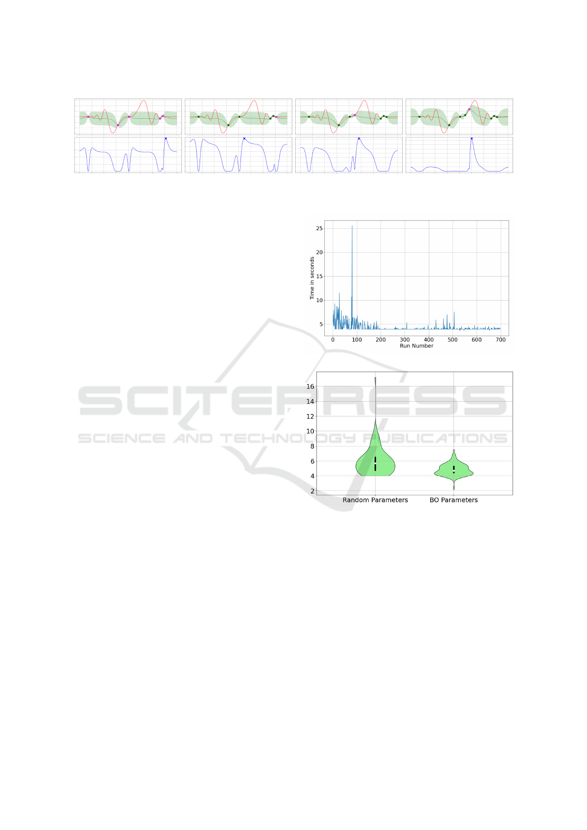
(a) Step 0. (b) Step 1. (c) Step 2. (d) Step 3.

Figure 2: An example of BO on an 1D objective function over 4 iterations.

ing here is that real-world motors are seldom perfect

systems. Due to friction, capacitor charges, etc. a lot

of inconsistency might occur. Thus, we chose a rela-

tively high rope to keep such inconsistencies in mind.

For the second objective, the motor ran for an ad-

ditional 10 seconds after speed up to measure the cur-

rent.

6.1 Single Objective

At ﬁrst, we focus on the angular acceleration. We

show the optimization progress as well as an empir-

ical comparison between random parameters and the

optimized one. For the last task, we compare 50 runs

each for statistical signiﬁcance.

The plain motor should be the simplest one to op-

timize as it does not include an axial impeller. The

other two motors should be more difﬁcult due to their

axial impeller.

As we can see in Figure 3a, the plain motor starts

with a high variance in time. Nonetheless, as op-

timization progresses, BO is able to ﬁnd good pa-

rameters. As for motor 2, we see a completely dif-

ferent history in Figure 4. There is a higher vari-

ance throughout the optimization progress with some

lower peaks. Thus one has to be critical of this op-

timization progress as there are high peaks through-

out the observations. For the last motor 3, the opti-

mization progress looks more promising in Figure 5a

compared to the second motor. It is able to periodi-

cally ﬁnd good values and we see a better optimiza-

tion progress.

An empirical comparison for the motors between

the best parameters found and random ones can be

seen in violin plots in Figure 3b, 4b and 5b. Here,

we compare the startup times between random pa-

rameters and the best parameters found by BO. We

can see that the random parameters take between 4

and > 10 seconds to speed up and most of the runs

take about ∼ 6 seconds for all motors. The optimized

parameters take on average between 4 and 5 seconds

but show a relatively high variance, too. Neverthe-

less, the variances of BO parameters are still lower

than random ones. Furthermore, it can be said that the

(a) Progression of BO.

(b) Random vs. best parameter found.

Figure 3: Progression of BO and an empirical comparison

given the plain motor.

optimized parameters behave better than the random

ones as they show a higher axial acceleration on av-

erage. This can be somewhat conﬁrmed by utilizing

BC. For the plain motor, the results are p

< 0.001,

= 0.407 and p

= 0.591. This shows us that our

found parameters are statistically better for about 59

percent of runs. However, these parameter sets are

statistically equal for about 41 percent. Motor 2 has

< 0.001, p

= 0.002 and p

= 0.998. On aver-

age, the best parameters found should be better than

random parameters. At last, motor 3 has a similar

behaviour. Here we get p

= 0.001, p

= 0.320 and

= 0.680. This tells us that both random parame-

ters and our BO parameters are statistically equal for

A Concept for Optimizing Motor Control Parameters Using Bayesian Optimization

111

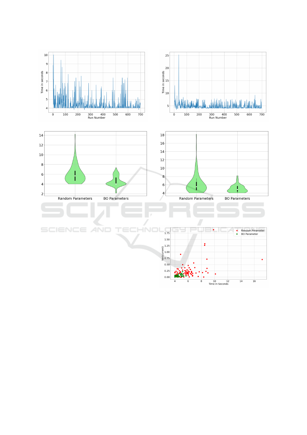
(a) Progression of BO.

(b) Random vs. best parameter found.

Figure 4: Progression of BO and an empirical comparison

given motor 2.

32 percent but statistically better for 68 percent.

6.2 Multi-Objective

At last, we try to optimize a multi-objective task de-

ﬁned in Section 4. Here, we ﬁguratively compare the

best parameter to random ones. For each compari-

son, we took 80 samples each and show a distribution

for Time in Seconds and Var(current). Furthermore,

we utilize the Hypervolume indicator (Zitzler et al.,

2008) to quantitatively compare our result.

6.2.1 Figurative Comparison

Looking at the plots in Figure 6, 7 and 8 for all three

motors, we see distributions of observations. They

contain data points from random parameters and the

parameters of the best solution found by the multi-

objective BO.

The coordinate system shows the variance of the

current ripple as well as the time it takes to speed up

in seconds. Green dots represent parameters found by

BO while red ones represent random ones. A lower

distance to the origin indicates a better parameter. We

can see that the random parameters are more scattered

(a) Progression of BO.

(b) Random vs. best parameter found.

Figure 5: Progression of BO and an empirical comparison

given motor 3.

Figure 6: Plain Motor: optimal parameter compared to ran-

dom ones. Lower distances to the origin are better.

throughout the coordinate system, indicating a high

variation. As for the plain motor and motor 2, we

see that the parameters found by the BO are more fo-

cused at the origin, indicating that those are superior

compared to the random parameter. However, Fig-

ure 6 still shows a slight variation for the BO parame-

ters which implies inconsistencies to some degree be-

tween each run.

As for motor 3, its evaluation results are more of

an outlier as is visualized in Figure 8. We see data

points of both the random and best parameters found

ICINCO 2023 - 20th International Conference on Informatics in Control, Automation and Robotics

112

Figure 7: Motor 2: optimal parameter compared to random

ones. Lower distances to the origin are better.

Figure 8: Motor 3: optimal parameter compared to random

ones. Lower distances to the origin are better.

scattered throughout the coordinate system. Given the

BO parameters, we can see that the runs are highly

inconsistent. Thus, it is likely that it is not possible to

optimize parameters for this speciﬁc setting.

6.2.2 Hypervolume Indicator

At last, we compare the found Pareto front with a

Pareto front generated from random search (RS). For

this comparison, we utilize the Hypervolume indica-

tor. Here, we calculate the volume bound by a ref-

erence point and the Pareto set containing all found

solutions. For the reference point, we choose a point

a little bit larger than the largest value found in both

axes as is recommended in (Beume et al., 2007).

Here, the greater the volume, the better the Pareto

front as a greater volume indicates a Pareto front

which is closer to the origin.

Our results can be seen in Table 1. We see that the

multi-objective BO ﬁnds better results for the plain

motor as well as motor 2 compared to a RS. How-

ever, motor 3 shows dissimilar results as the RS out-

performs the multi-objective BO here. Nevertheless,

the difference is only marginal and it can be argued

that both Pareto sets are equally good.

Table 1: Hypervolume indicators for each motor and Pareto

front.

Pareto Front Plain Motor Motor 2 Motor 3

Found by BO 42.68 35.31 94.19

Found by RS 40.93 33.84 94.27

7 CONCLUSION

Throughout our work we performed the ﬁrst steps into

automating this process. We provide insight into a

possible hardware test bed and how it may be con-

trolled. Our key contribution is development of an

optimization routine based on Bayesian Optimization

(BO) which calibrates up to two motor properties in

parallel.

Our evaluation shows mixed results. Generally,

there is a trend towards a highly inconsistent setting,

as the same parameter can create different evaluation

values. Thus, the ﬂuctuating results demonstrate a

complex objective for the BO. However, BO is able

to ﬁnd good parameters most of the time and we are

able to successfully statistically compare our results

to random ones most of the times.

For future work, other acquisition functions as

well as kernels for the GP function might result in

better products. When adjusted to our problem do-

main to consider the non-deterministic nature of the

motors, Bayesian Optimization might be able to pro-

duce better results.

ACKNOWLEDGEMENTS

The authors would like to thank Tomas Hrubov-

cak, Martin Gula and Slavomir Maciboba from BSH

Drives and Pumps s.r.o. in Michalovce, Slovakia.

Their numerous and detailed help made a functioning

testbed possible.

REFERENCES

Akrour, R., Sorokin, D., Peters, J., and Neumann, G.

(2017). Local bayesian optimization of motor skills.

In International Conference on Machine Learning,

pages 41–50. PMLR.

Benavoli, A., Corani, G., Dem

sar, J., and Zaffalon, M.

(2017). Time for a change: a tutorial for compar-

ing multiple classiﬁers through bayesian analysis. The

Journal of Machine Learning Research, 18(1):2653–

2688.

Beume, N., Naujoks, B., and Emmerich, M. (2007). Sms-

emoa: Multiobjective selection based on dominated

A Concept for Optimizing Motor Control Parameters Using Bayesian Optimization

113

hypervolume. European Journal of Operational Re-

search, 181(3):1653–1669.

Brochu, E., Cora, V. M., and de Freitas, N. (2009). A tuto-

rial on bayesian optimization of expensive cost func-

tions, with application to active user modeling and hi-

erarchical reinforcement learning. Technical Report

UBC TR-2009-023 and arXiv:1012.2599, University

of British Columbia, Department of Computer Sci-

ence. http://arxiv.org/abs/1012.2599/.

Buitinck, L., Louppe, G., Blondel, M., Pedregosa, F.,

Mueller, A., Grisel, O., Niculae, V., Prettenhofer, P.,

Gramfort, A., Grobler, J., Layton, R., VanderPlas, J.,

Joly, A., Holt, B., and Varoquaux, G. (2013). API de-

sign for machine learning software: experiences from

the scikit-learn project. In ECML PKDD Workshop:

Languages for Data Mining and Machine Learning,

pages 108–122.

Cox, D. D. and John, S. (1992). A statistical method for

global optimization. In [Proceedings] 1992 IEEE In-

ternational Conference on Systems, Man, and Cyber-

netics, pages 1241–1246. IEEE.

Deb, K., Pratap, A., Agarwal, S., and Meyarivan, T. (2002).

A fast and elitist multiobjective genetic algorithm:

Nsga-ii. IEEE Transactions on Evolutionary Compu-

tation, 6(2):182–197.

Ehrgott, M. (2005). Multicriteria optimization, volume 491.

Springer Science & Business Media.

Frazier, P. I. (2018). A tutorial on bayesian optimization.

https://arxiv.org/abs/1807.02811/.

Galuzio, P. P., de Vasconcelos Segundo, E. H., dos San-

tos Coelho, L., and Mariani, V. C. (2020). Mobopt

— multi-objective bayesian optimization. SoftwareX,

12:100520.

Ghazali, M. R., Ahmad, M. A., Suid, M. H., and Tumari, M.

Z. M. (2022). A dc/dc buck-boost converter-inverter-

dc motor control based on model-free pid controller

tuning by adaptive safe experimentation dynamics al-

gorithm. In 2022 57th International Universities

Power Engineering Conference (UPEC), pages 1–6.

Jones, D. R. (2001). A taxonomy of global optimiza-

tion methods based on response surfaces. Journal of

Global Optimization, 21(4):345–383.

Jones, D. R., Schonlau, M., and Welch, W. J. (1998).

Efﬁcient global optimization of expensive black-

box functions. Journal of Global Optimization,

13(4):455–492.

Kaminski, M. (2020). Nature-inspired algorithm imple-

mented for stable radial basis function neural con-

troller of electric drive with induction motor. Ener-

gies, 13(24).

Khosravi, M., Behrunani, V. N., Myszkorowski, P.,

Smith, R. S., Rupenyan, A., and Lygeros, J. (2021).

Performance-driven cascade controller tuning with

bayesian optimization. IEEE Transactions on Indus-

trial Electronics, 69(1):1032–1042.

Kushner, H. J. (1964). A New Method of Locating the

Maximum Point of an Arbitrary Multipeak Curve in

the Presence of Noise. Journal of Basic Engineering,

86(1):97–106.

onig, C., Turchetta, M., Lygeros, J., Rupenyan, A., and

Krause, A. (2021). Safe and efﬁcient model-free adap-

tive control via bayesian optimization. In 2021 IEEE

International Conference on Robotics and Automation

(ICRA), pages 9782–9788.

Magtrol Inc. (2022a). Dsp7000 – high speed programmable

controller. https://www.magtrol.com/product/

dsp7000-high-speed-programmable-controller/,

Accessed: 2022-07-15.

Magtrol Inc. (2022b). Hd series – hysteresis dy-

namometers. https://www.magtrol.com/product/

hysteresis-dynamometers-hd-series/, Accessed:

2022-07-15.

Mockus, J. (1975). On bayesian methods for seeking the

extremum. In Marchuk, G. I., editor, Optimization

Techniques IFIP Technical Conference Novosibirsk,

July 1–7, 1974, pages 400–404, Berlin, Heidelberg.

Springer Berlin Heidelberg.

Mockus, J. (2012). Bayesian approach to global optimiza-

tion: theory and applications, volume 37. Springer

Science & Business Media.

Naidu Kommula, B. and Reddy Kota, V. (2022). Design of

mfa-pso based fractional order pid controller for effec-

tive torque controlled bldc motor. Sustainable Energy

Technologies and Assessments, 49:101644.

Neumann-Brosig, M., Marco, A., Schwarzmann, D., and

Trimpe, S. (2020). Data-efﬁcient autotuning with

bayesian optimization: An industrial control study.

IEEE Transactions on Control Systems Technology,

28(3):730–740.

Ngatchou, P., Zarei, A., and El-Sharkawi, A. (2005). Pareto

multi objective optimization. In Proceedings of the

13th International Conference on, Intelligent Systems

Application to Power Systems, pages 84–91.

Rasmussen, C. E. (2003). Gaussian processes in machine

learning. In Summer school on machine learning,

pages 63–71. Springer.

Shahriari, B., Swersky, K., Wang, Z., Adams, R. P., and

de Freitas, N. (2016). Taking the human out of the

loop: A review of bayesian optimization. Proceedings

of the IEEE, 104(1):148–175.

Sharma, A., Sharma, V., and Rahi, O. P. (2022). Pso tuned

pid controller for dc motor speed control. In Suhag,

S., Mahanta, C., and Mishra, S., editors, Control and

Measurement Applications for Smart Grid, pages 79–

89, Singapore. Springer Nature Singapore.

Snoek, J., Larochelle, H., and Adams, R. P. (2012). Practi-

cal bayesian optimization of machine learning algo-

rithms. In Pereira, F., Burges, C., Bottou, L., and

Weinberger, K., editors, Advances in Neural Infor-

mation Processing Systems, volume 25. Curran Asso-

ciates, Inc.

Tarczewski, T. and Grzesiak, L. M. (2018). An applica-

tion of novel nature-inspired optimization algorithms

to auto-tuning state feedback speed controller for

pmsm. IEEE Transactions on Industry Applications,

54(3):2913–2925.

Zitzler, E., Knowles, J., and Thiele, L. (2008). Quality

Assessment of Pareto Set Approximations. Springer

Berlin Heidelberg, Berlin, Heidelberg.

ICINCO 2023 - 20th International Conference on Informatics in Control, Automation and Robotics

114